Page 247 - Computational Statistics Handbook with MATLAB

Chapter 7: Data Partitioning 235

observed x values, the observed y values and the degree of the polynomial
that we want to fit to the data. The following commands fit a polynomial of
degree one to the steam data.
% Loads the vectors x and y.
load steam
% Fit a first degree polynomial to the data.
[p,s] = polyfit(x,y,1);
The output argument p is a vector of coefficients of the polynomial in
decreasing order. So, in this case, the first element of p is the estimated slope
ˆ ˆ The resulting
β 1 and the second element is the estimated y-intercept β 0 .
model is
ˆ ˆ
β 0 = 13.62 β 1 = – 0.08 .

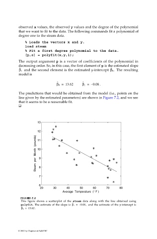
The predictions that would be obtained from the model (i.e., points on the
line given by the estimated parameters) are shown in Figure 7.2, and we see
that it seems to be a reasonable fit.

13

12
Steam per Month (pounds) 10
11

9

8

7

6
20 30 40 50 60 70 80
Average Temperature ( ° F )

GU
U
F FI F F II IG URE G 7. RE RE RE 7. 7. 7. 2 2
2
2
GU
This figure shows a scatterplot of the steam data along with the line obtained using
ˆ
polyfit. The estimate of the slope is β 1 = – 0.08, and the estimate of the y-intercept is
ˆ
β 0 = 13.62 .
© 2002 by Chapman & Hall/CRC