Page 245 - Computational Statistics Handbook with MATLAB

Chapter 7: Data Partitioning 233

with data it has already seen. Therefore, that procedure will yield an overly
optimistic (i.e., low) prediction error (see Equation 7.5). Cross-validation is a
technique that can be used to address this problem by iteratively partitioning
the sample into two sets of data. One is used for building the model, and the
other is used to test it.
We introduce cross-validation in a linear regression application, where we
are interested in estimating the expected prediction error. We use linear
regression to illustrate the cross-validation concept, because it is a topic that
most engineers and data analysts should be familiar with. However, before
we describe the details of cross-validation, we briefly review the concepts in
linear regression. We will return to this topic in Chapter 10, where we discuss
methods of nonlinear regression.
(
,
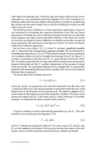
Say we have a set of data, X i Y i ) , where X i denotes a predictor variable
represents the corresponding response variable. We are interested in
and Y i
modeling the dependency of Y on X. The easiest example of linear regression
is in situations where we can fit a straight line between X and Y. In Figure 7.1,
(
we show a scatterplot of 25 observed X i Y i ) pairs [Draper and Smith, 1981].
,
The X variable represents the average atmospheric temperature measured in
degrees Fahrenheit, and the Y variable corresponds to the pounds of steam
used per month. The scatterplot indicates that a straight line is a reasonable
model for the relationship between these variables. We will use these data to
illustrate linear regression.
The linear, first-order model is given by

Y = β 0 + β 1 X + , ε (7.1)

are parameters that must be estimated from the data, and
where β 0 and β 1
ε represents the error in the measurements. It should be noted that the word
. The order (or degree) of the
linear refers to the linearity of the parameters β i
model refers to the highest power of the predictor variable X. We know from
is the y-intercept. As another
elementary algebra that β 1 is the slope and β 0
example, we represent the linear, second-order model by

2
Y = β 0 + β 1 X + β 2 X + ε . (7.2)

. Thus, the
To get the model, we need to estimate the parameters β 0 and β 1
estimate of our model given by Equation 7.1 is
ˆ ˆ ˆ
Y = β 0 + β 1X , (7.3)
ˆ ˆ
where Y denotes the predicted value of Y for some value of X, and β 0 and
ˆ
β 1 are the estimated parameters. We do not go into the derivation of the esti-
mators, since it can be found in most introductory statistics textbooks.

© 2002 by Chapman & Hall/CRC