Page 246 - Computational Statistics Handbook with MATLAB

234 Computational Statistics Handbook with MATLAB

13

12
Steam per Month (pounds) 10
11

9

8

7

6
20 30 40 50 60 70 80
Average Temperature ( ° F )
FI F IG URE G 7. RE 7. 1 1
U
GU
F F II GU RE RE 7. 7. 1
1
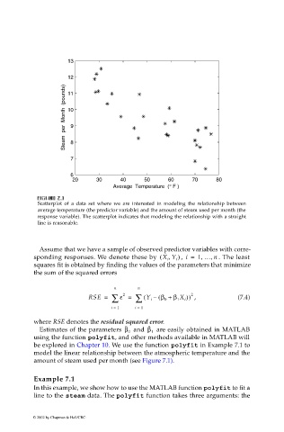
Scatterplot of a data set where we are interested in modeling the relationship between
average temperature (the predictor variable) and the amount of steam used per month (the
response variable). The scatterplot indicates that modeling the relationship with a straight
line is reasonable.
Assume that we have a sample of observed predictor variables with corre-
(
,
,
,
sponding responses. We denote these by X i Y i ) i = 1 … n . The least
,
squares fit is obtained by finding the values of the parameters that minimize
the sum of the squared errors
n n
2
RSE = ∑ ε = ∑ ( Y i – ( β 0 + β 1 X i )) 2 , (7.4)
i = 1 i = 1
where RSE denotes the residual squared error.
ˆ ˆ
Estimates of the parameters β 0 and β 1 are easily obtained in MATLAB
using the function polyfit, and other methods available in MATLAB will
be explored in Chapter 10. We use the function polyfit in Example 7.1 to
model the linear relationship between the atmospheric temperature and the
amount of steam used per month (see Figure 7.1).

Example 7.1
In this example, we show how to use the MATLAB function polyfit to fit a
line to the steam data. The polyfit function takes three arguments: the

© 2002 by Chapman & Hall/CRC