Page 249 - Computational Statistics Handbook with MATLAB

Chapter 7: Data Partitioning 237

xtrain(indtest) = [];
ytrain(indtest) = [];
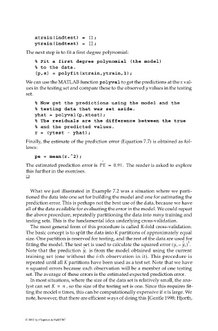
The next step is to fit a first degree polynomial:

% Fit a first degree polynomial (the model)
% to the data.
[p,s] = polyfit(xtrain,ytrain,1);
We can use the MATLAB function polyval to get the predictions at the x val-
ues in the testing set and compare these to the observed y values in the testing
set.

% Now get the predictions using the model and the
% testing data that was set aside.
yhat = polyval(p,xtest);
% The residuals are the difference between the true
% and the predicted values.
r = (ytest - yhat);
Finally, the estimate of the prediction error (Equation 7.7) is obtained as fol-
lows:

pe = mean(r.^2);
ˆ
The estimated prediction error is PE = 0.91. The reader is asked to explore
this further in the exercises.

What we just illustrated in Example 7.2 was a situation where we parti-
tioned the data into one set for building the model and one for estimating the
prediction error. This is perhaps not the best use of the data, because we have
all of the data available for evaluating the error in the model. We could repeat
the above procedure, repeatedly partitioning the data into many training and
testing sets. This is the fundamental idea underlying cross-validation.
The most general form of this procedure is called K-fold cross-validation.
The basic concept is to split the data into K partitions of approximately equal
size. One partition is reserved for testing, and the rest of the data are used for
2
fitting the model. The test set is used to calculate the squared error y i –( y i ) .
ˆ
ˆ
Note that the prediction y i is from the model obtained using the current
training set (one without the i-th observation in it). This procedure is
repeated until all K partitions have been used as a test set. Note that we have
n squared errors because each observation will be a member of one testing
set. The average of these errors is the estimated expected prediction error.
In most situations, where the size of the data set is relatively small, the ana-
lyst can set K = n , so the size of the testing set is one. Since this requires fit-
ting the model n times, this can be computationally expensive if n is large. We
note, however, that there are efficient ways of doing this [Gentle 1998; Hjorth,

© 2002 by Chapman & Hall/CRC