Page 252 - Computational Statistics Handbook with MATLAB

240 Computational Statistics Handbook with MATLAB

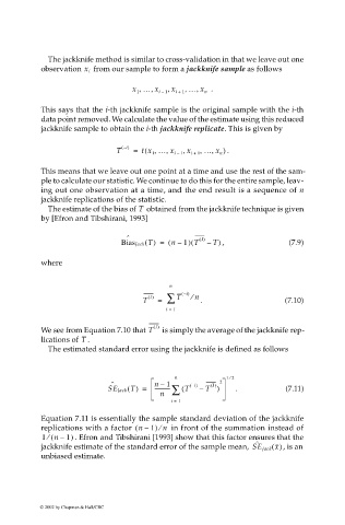
The jackknife method is similar to cross-validation in that we leave out one
from our sample to form a jackknife sample as follows
observation x i
x … x, , x , , … x .
,
1 i – 1 i + 1 n
This says that the i-th jackknife sample is the original sample with the i-th
data point removed. We calculate the value of the estimate using this reduced
jackknife sample to obtain the i-th jackknife replicate. This is given by

i – ()
T = tx 1 … x i – ,( , , 1 x i + , , . )
1 … x n
This means that we leave out one point at a time and use the rest of the sam-
ple to calculate our statistic. We continue to do this for the entire sample, leav-
ing out one observation at a time, and the end result is a sequence of n
jackknife replications of the statistic.
The estimate of the bias of obtained from the jackknife technique is given
T
by [Efron and Tibshirani, 1993]
ˆ J ()
(
Bias Jack T() = ( n – ) T – T) , (7.9)
1
where

n
J () ∑ T i – () n ⁄
T = . (7.10)
i = 1
J ()
We see from Equation 7.10 that T is simply the average of the jackknife rep-
T
lications of .
The estimated standard error using the jackknife is defined as follows

⁄
n 12
ˆ n – 1 i – () J () 2
SE Jack T() = ------------ ∑ ( T – T ) . (7.11)
n
i = 1
Equation 7.11 is essentially the sample standard deviation of the jackknife
replications with a factor n –( 1) n in front of the summation instead of
⁄
1 ( n – 1) . Efron and Tibshirani [1993] show that this factor ensures that the
⁄
ˆ
jackknife estimate of the standard error of the sample mean, SE Jack x() , is an
unbiased estimate.

© 2002 by Chapman & Hall/CRC