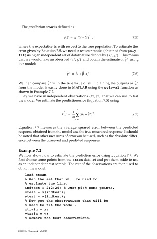
Page 248 - Computational Statistics Handbook with MATLAB

236 Computational Statistics Handbook with MATLAB

The prediction error is defined as

ˆ
( [
PE = E Y – Y) 2 , ] (7.5)
where the expectation is with respect to the true population. To estimate the
error given by Equation 7.5, we need to test our model (obtained from poly-
fit) using an independent set of data that we denote by x i ' y i ',( ) . This means
that we would take an observed x i ' y i ',( ) and obtain the estimate of y i ' using
ˆ
our model:

ˆ
ˆ
ˆ
y i ' = β 0 + β 1x i . ' (7.6)
ˆ
ˆ
We then compare y i ' with the true value of y ' . Obtaining the outputs or y i '
i
from the model is easily done in MATLAB using the polyval function as
shown in Example 7.2.
Say we have m independent observations x ' y ',( ) that we can use to test
i i
the model. We estimate the prediction error (Equation 7.5) using
m
ˆ 1 ˆ 2
PE = ---- ∑ ( y i ' – y i ') . (7.7)
m
i = 1
Equation 7.7 measures the average squared error between the predicted
response obtained from the model and the true measured response. It should
be noted that other measures of error can be used, such as the absolute differ-
ence between the observed and predicted responses.

Example 7.2
We now show how to estimate the prediction error using Equation 7.7. We
first choose some points from the steam data set and put them aside to use
as an independent test sample. The rest of the observations are then used to
obtain the model.

load steam
% Get the set that will be used to
% estimate the line.
indtest = 2:2:20; % Just pick some points.
xtest = x(indtest);
ytest = y(indtest);
% Now get the observations that will be
% used to fit the model.
xtrain = x;
ytrain = y;
% Remove the test observations.

© 2002 by Chapman & Hall/CRC