Page 261 - Computational Statistics Handbook with MATLAB

Chapter 7: Data Partitioning 249

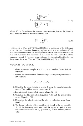
n  3
i)
∑  θ ˆ J() – θ ˆ –( 



ˆ a = ------------------------------------------------------- , (7.19)
i =
1
⁄
 n 2  32
6  ∑  θ ˆ J() – θ ˆ –() i  
   
i = 1
where θ ˆ –( i) is the value of the statistic using the sample with the i-th data
point removed (the i-th jackknife sample) and
n
ˆ J()
θ = 1 ∑ θ ˆ –( i) . (7.20)
---
n
i = 1
ˆ
According to Efron and Tibshirani [1993], z 0 is a measure of the difference
ˆ
θ
between the median of the bootstrap replicates and in normal units. If half
θ
ˆ
of the bootstrap replicates are less than or equal to , then there is no median
ˆ ˆ
a
bias and z 0 is zero. The parameter measures the rate acceleration of the
θ
ˆ
standard error of . For more information on the theoretical justification for
these corrections, see Efron and Tibshirani [1993] and Efron [1987].
INTERVAL
PROCEDURE - BC a
,
,
1. Given a random sample, x = ( x 1 … x n ) , calculate the statistic of
θ
ˆ
interest .
2. Sample with replacement from the original sample to get the boot-
strap sample
,
,
*b
x *b = ( x 1 … x n *b . )
3. Calculate the same statistic as in step 1 using the sample found in
step 2. This yields a bootstrap replicate θ ˆ *b .
4. Repeat steps 2 through 3, B times, where B ≥ 1000 .
5. Calculate the bias correction (Equation 7.18) and the acceleration
factor (Equation 7.19).
6. Determine the adjustments for the interval endpoints using Equa-
tion 7.17.
quantile
7. The lower endpoint of the confidence interval is the α 1
ˆ
q α of the bootstrap replicates, and the upper endpoint of the
1
ˆ
confidence interval is the α 2 quantile q α of the bootstrap repli-
2
cates.

© 2002 by Chapman & Hall/CRC