Page 260 - Computational Statistics Handbook with MATLAB

248 Computational Statistics Handbook with MATLAB

(
(
ˆ
ˆ
1 ˆ
,
(
2
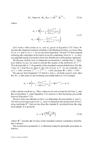
Interval: θLo θHi) = ( ˆ * α ) , * α ) , ) (7.16)
BC a θ B θB
where
 z 0 + z ( α 2) 
⁄
ˆ
ˆ

α 1 = Φ z 0 + ----------------------------------------
⁄
 1 – ˆ ˆ z ( α 2) )
a z 0 +(
(7.17)
 ˆ z 0 + z ( 1 – α 2) 
⁄
ˆ

α = Φ z 0 + ---------------------------------------------- .
2
⁄
ˆ ˆ
 1 – a z 0 +( z ( 1 – α 2) )
given in Equation 7.17. Since Φ
Let’s look a little closer at α 1 and α 2
denotes the standard normal cumulative distribution function, we know that
0 ≤ α 1 ≤ 1 and 0 ≤ α 2 ≤ 1 . So we see from Equation 7.16 and 7.17 that instead
of basing the endpoints of the interval on the confidence level of 1 – α , they
are adjusted using information from the distribution of bootstrap replicates.
a ˆ ˆ . How-
We discuss, shortly, how to obtain the acceleration and the bias z 0
( α 2)
⁄
ever, before we do, we want to remind the reader of the definition of z .
This denotes the α 2⁄ -th quantile of the standard normal distribution. It is the
value of z that has an area to the left of size α 2⁄ . As an example, for
⁄
⁄
α 2 = 0.05 , we have z ( α 2) = z ( 0.05) = – 1.645 , because Φ –( 1.645) = 0.05 .
ˆ ˆ
a
We can see from Equation 7.17 that if and z 0 are both equal to zero, then
is the same as the bootstrap percentile interval. For example,
the BC a
 0 + z ( α 2)  ( α 2)
⁄
⁄

α 1 = Φ 0 + ---------------------------------------  = Φ z ( ) = α , 2 ⁄
⁄
 1 – 0 0 +( z ( α 2) )
ˆ
with a similar result for α 2 . Thus, when we do not account for the bias z 0 and
ˆ
the acceleration , then Equation 7.16 reduces to the bootstrap percentile
a
interval (Equation 7.15).
ˆ ˆ
a
We now turn our attention to how we determine the parameters and z 0 .
ˆ
The bias-correction is given by z 0 , and it is based on the proportion of boot-
strap replicates θ ˆ *b that are less than the statistic calculated from the orig-
θ
ˆ
inal sample. It is given by
ˆ
ˆ *b
θ)
1 # θ <(
ˆ
z 0 = Φ –  ------------------------  , (7.18)
 B 
where Φ – 1 denotes the inverse of the standard normal cumulative distribu-
tion function.
ˆ
a
The acceleration parameter is obtained using the jackknife procedure as
follows,
© 2002 by Chapman & Hall/CRC