Page 97 - Computational Statistics Handbook with MATLAB

84 Computational Statistics Handbook with MATLAB

1
0.73

0.8

F(X) 0.6

0.4

0.2

0
0 1 2 0
X

IG
F FI U URE G 4. RE 4. 2 2
GU
2
F F II GU RE RE 4. 4. 2
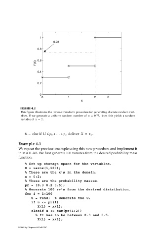
This figure illustrates the inverse transform procedure for generating discrete random vari-
ables. If we generate a uniform random number of u = 0.73, then this yields a random
variable of x = 2 .
6. ... else if U ≤ p 0 + … + p k deliver X = x k .

Example 4.3
We repeat the previous example using this new procedure and implement it
in MATLAB. We first generate 100 variates from the desired probability mass
function.

% Set up storage space for the variables.
X = zeros(1,100);
% These are the x's in the domain.
x = 0:2;
% These are the probability masses.
pr = [0.3 0.2 0.5];
% Generate 100 rv’s from the desired distribution.
for i = 1:100
u = rand; % Generate the U.
if u <= pr(1)
X(i) = x(1);
elseif u <= sum(pr(1:2))
% It has to be between 0.3 and 0.5.
X(i) = x(2);

© 2002 by Chapman & Hall/CRC