Page 99 - Computational Statistics Handbook with MATLAB

86 Computational Statistics Handbook with MATLAB

PROCEDURE - ACCEPTANCE-REJECTION METHOD (CONTINUOUS)
1. Choose a density gy() that is easy to sample from.

2. Find a constant c such that Equation 4.6 is satisfied.
3. Generate a random number Y from the density gy() .
4. Generate a uniform random number U.
5. If

fY()
U ≤ --------------- ,
cg Y()

then accept X = Y , else go to step 3.

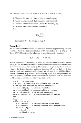
Example 4.4
We shall illustrate the acceptance-rejection method by generating random
variables from the beta distribution with parameters α = 2 and β = 1
[Ross, 1997]. This yields the following probability density function

f x() = 2x; 0 < x < . 1 (4.7)

Since the domain of this density is 0 to 1, we use the uniform distribution for
our gy() . We must find a constant that we can use to inflate the uniform so it
is above the desired beta density. This constant is given by the maximum
value of the density function, and from Equation 4.7, we see that c = 2 . For
more complicated functions, techniques from calculus or the MATLAB func-
tion fminsearch may be used. The following MATLAB code generates 100
random variates from the desired distribution. We save both the accepted
and the rejected variates for display purposes only.

c = 2; % constant
n = 100; % Generate 100 random variables.
% Set up the arrays to store variates.
x = zeros(1,n); % random variates
xy = zeros(1,n);% corresponding y values
rej = zeros(1,n);% rejected variates
rejy = zeros(1,n); % corresponding y values
irv = 1;
irej = 1;
while irv <= n
y = rand(1); % random number from g(y)
u = rand(1); % random number for comparison
if u <= 2*y/c;
x(irv) = y;
xy(irv) = u*c;

© 2002 by Chapman & Hall/CRC