Page 112 -

3.1 Point operators 91

160
45 60 98 127 132 133 137 133 140
120
46 65 98 123 126 128 131 133
100
47 65 96 115 119 123 135 137 range 80
47 63 91 107 113 122 138 134 60
50 59 80 97 110 123 133 134 40
20
49 53 68 83 97 113 128 133 0 15
50 50 58 70 84 102 116 126 S16 S15 S14 S13 S12 S11 9 11 domain 13
domain S10 S9 S8 S7 S6 5 7
50 50 52 58 69 86 101 120 S5 S4 S3 S2 S1 1 3
(a) (b) (c) (d)
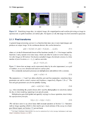
Figure 3.3 Visualizing image data: (a) original image; (b) cropped portion and scanline plot using an image in-
spection tool; (c) grid of numbers; (d) surface plot. For figures (c)–(d), the image was first converted to grayscale.

3.1.1 Pixel transforms

A general image processing operator is a function that takes one or more input images and
produces an output image. In the continuous domain, this can be denoted as

g(x)= h(f(x)) or g(x)= h(f 0 (x),...,f n (x)), (3.1)
where x is in the D-dimensional domain of the functions (usually D =2 for images) and the
functions f and g operate over some range, which can either be scalar or vector-valued, e.g.,
for color images or 2D motion. For discrete (sampled) images, the domain consists of a finite
number of pixel locations, x =(i, j), and we can write

g(i, j)= h(f(i, j)). (3.2)

Figure 3.3 shows how an image can be represented either by its color (appearance), as a grid
of numbers, or as a two-dimensional function (surface plot).
Two commonly used point processes are multiplication and addition with a constant,
g(x)= af(x)+ b. (3.3)

The parameters a> 0 and b are often called the gain and bias parameters; sometimes these
1
parameters are said to control contrast and brightness, respectively (Figures 3.2b–c). The
bias and gain parameters can also be spatially varying,
g(x)= a(x)f(x)+ b(x), (3.4)

e.g., when simulating the graded density filter used by photographers to selectively darken
the sky or when modeling vignetting in an optical system.
Multiplicative gain (both global and spatially varying) is a linear operation, since it obeys
the superposition principle,
h(f 0 + f 1 )= h(f 0 )+ h(f 1 ). (3.5)

(We will have more to say about linear shift invariant operators in Section 3.2.) Operators
such as image squaring (which is often used to get a local estimate of the energy in a band-
pass filtered signal, see Section 3.5) are not linear.

1 An image’s luminance characteristics can also be summarized by its key (average luminanance) and range
(Kopf, Uyttendaele, Deussen et al. 2007).