Page 116 -

3.1 Point operators 95

6000 350000
B B
5000 G 300000 G
R 250000 R
4000
Y Y
200000
3000
150000
2000
100000
1000 50000
0 0
0 50 100 150 200 250 0 50 100 150 200 250
(a) (b) (c)
250
B
200 G
R
150 Y
100
50
0
0 50 100 150 200 250
(d) (e) (f)
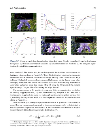
Figure 3.7 Histogram analysis and equalization: (a) original image (b) color channel and intensity (luminance)
histograms; (c) cumulative distribution functions; (d) equalization (transfer) functions; (e) full histogram equal-
ization; (f) partial histogram equalization.

these heuristics? The answer is to plot the histogram of the individual color channels and
2
luminance values, as shown in Figure 3.7b. From this distribution, we can compute relevant
statistics such as the minimum, maximum, and average intensity values. Notice that the image
in Figure 3.7a has both an excess of dark values and light values, but that the mid-range values
are largely under-populated. Would it not be better if we could simultaneously brighten some
dark values and darken some light values, while still using the full extent of the available
dynamic range? Can you think of a mapping that might do this?
One popular answer to this question is to perform histogram equalization, i.e., to find
an intensity mapping function f(I) such that the resulting histogram is flat. The trick to
finding such a mapping is the same one that people use to generate random samples from
a probability density function, which is to first compute the cumulative distribution function
shown in Figure 3.7c.
Think of the original histogram h(I) as the distribution of grades in a class after some
exam. How can we map a particular grade to its corresponding percentile, so that students at
the 75% percentile range scored better than / 4 of their classmates? The answer is to integrate
3
the distribution h(I) to obtain the cumulative distribution c(I),
I
1 1
c(I)= h(i)= c(I − 1) + h(I), (3.9)
N N
i=0
2
The histogram is simply the count of the number of pixels at each gray level value. For an eight-bit image, an
accumulation table with 256 entries is needed. For higher bit depths, a table with the appropriate number of entries
(probably fewer than the full number of gray levels) should be used.