Page 119 -

98 3 Image processing

45 60 98 127 132 133 137 133
46 65 98 123 126 128 131 133 69 95 116 125 129 132
47 65 96 115 119 123 135 137 0.1 0.1 0.1 68 92 110 120 126 132
47 63 91 107 113 122 138 134 * 0.1 0.2 0.1 = 66 86 104 114 124 132
50 59 80 97 110 123 133 134 0.1 0.1 0.1 62 78 94 108 120 129
49 53 68 83 97 113 128 133 57 69 83 98 112 124
50 50 58 70 84 102 116 126 53 60 71 85 100 114
50 50 52 58 69 86 101 120

f (x,y ) h (x,y ) g (x,y )

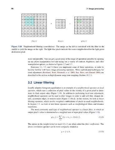
Figure 3.10 Neighborhood filtering (convolution): The image on the left is convolved with the filter in the
middle to yield the image on the right. The light blue pixels indicate the source neighborhood for the light green
destination pixel.

more interpretable. You can get a good sense of the range of operations possible by opening
up any photo manipulation tool and trying out a variety of contrast, brightness, and color
manipulation options, as shown in Figures 3.2 and 3.7.
Exercises 3.1, 3.5, and 3.6 have you implement some of these operations, in order to
become familiar with basic image processing operators. More sophisticated techniques for
tonal adjustment (Reinhard, Ward, Pattanaik et al. 2005; Bae, Paris, and Durand 2006) are
described in the section on high dynamic range tone mapping (Section 10.2.1).

3.2 Linear filtering

Locally adaptive histogram equalization is an example of a neighborhood operator or local
operator, which uses a collection of pixel values in the vicinity of a given pixel to deter-
mine its final output value (Figure 3.10). In addition to performing local tone adjustment,
neighborhood operators can be used to filter images in order to add soft blur, sharpen de-
tails, accentuate edges, or remove noise (Figure 3.11b–d). In this section, we look at linear
filtering operators, which involve weighted combinations of pixels in small neighborhoods.
In Section 3.3, we look at non-linear operators such as morphological filters and distance
transforms.
The most commonly used type of neighborhood operator is a linear filter, in which an
output pixel’s value is determined as a weighted sum of input pixel values (Figure 3.10),

g(i, j)= f(i + k, j + l)h(k, l). (3.12)
k,l
The entries in the weight kernel or mask h(k, l) are often called the filter coefficients. The
above correlation operator can be more compactly notated as

g = f ⊗ h. (3.13)