Page 121 -

100 3 Image processing

⎡ ⎤ ⎡ ⎤
21 . . . 72
⎢ 121 . . ⎥ ⎢ 88 ⎥
⎥ ⎢
⎢
⎥
⎢ .
72 88 62 52 37 ∗ 1 / 4 1 / 2 1 / 4 ⇔ 1 ⎢ 121 ⎥ ⎢ ⎥
4 . ⎥ ⎢ 62 ⎥
⎣ . . 121 ⎦ ⎣ 52 ⎦
⎥
⎥ ⎢
⎢
. . . 12 37
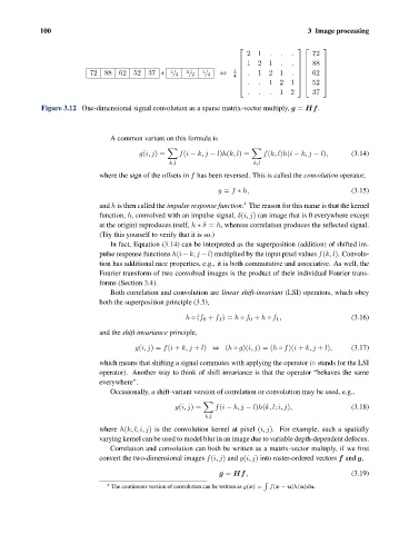
Figure 3.12 One-dimensional signal convolution as a sparse matrix-vector multiply, g = Hf.
A common variant on this formula is

g(i, j)= f(i − k, j − l)h(k, l)= f(k, l)h(i − k, j − l), (3.14)
k,l k,l
where the sign of the offsets in f has been reversed. This is called the convolution operator,
g = f ∗ h, (3.15)

4
and h is then called the impulse response function. The reason for this name is that the kernel
function, h, convolved with an impulse signal, δ(i, j) (an image that is 0 everywhere except
at the origin) reproduces itself, h ∗ δ = h, whereas correlation produces the reflected signal.
(Try this yourself to verify that it is so.)
In fact, Equation (3.14) can be interpreted as the superposition (addition) of shifted im-
pulse response functions h(i−k, j −l) multiplied by the input pixel values f(k, l). Convolu-
tion has additional nice properties, e.g., it is both commutative and associative. As well, the
Fourier transform of two convolved images is the product of their individual Fourier trans-
forms (Section 3.4).
Both correlation and convolution are linear shift-invariant (LSI) operators, which obey
both the superposition principle (3.5),

h ◦ (f 0 + f 1 )= h ◦ f 0 + h ◦ f 1 , (3.16)

and the shift invariance principle,
g(i, j)= f(i + k, j + l) ⇔ (h ◦ g)(i, j)=(h ◦ f)(i + k, j + l), (3.17)

which means that shifting a signal commutes with applying the operator (◦ stands for the LSI
operator). Another way to think of shift invariance is that the operator “behaves the same
everywhere”.
Occasionally, a shift-variant version of correlation or convolution may be used, e.g.,

g(i, j)= f(i − k, j − l)h(k, l; i, j), (3.18)
k,l
where h(k, l; i, j) is the convolution kernel at pixel (i, j). For example, such a spatially
varying kernel can be used to model blur in an image due to variable depth-dependent defocus.
Correlation and convolution can both be written as a matrix-vector multiply, if we first
convert the two-dimensional images f(i, j) and g(i, j) into raster-ordered vectors f and g,
g = Hf, (3.19)

4 The continuous version of convolution can be written as g(x)= f(x − u)h(u)du.