Page 118 -

3.1 Point operators 97

s s

t
t

(a) (b)

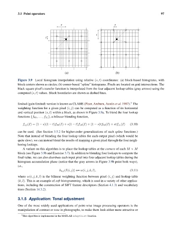
Figure 3.9 Local histogram interpolation using relative (s, t) coordinates: (a) block-based histograms, with
block centers shown as circles; (b) corner-based “spline” histograms. Pixels are located on grid intersections. The
black square pixel’s transfer function is interpolated from the four adjacent lookup tables (gray arrows) using the
computed (s, t) values. Block boundaries are shown as dashed lines.

3
limited (gain-limited) version is known as CLAHE (Pizer, Amburn, Austin et al. 1987). The
weighting function for a given pixel (i, j) can be computed as a function of its horizontal
and vertical position (s, t) within a block, as shown in Figure 3.9a. To blend the four lookup
functions {f 00 ,...,f 11 },a bilinear blending function,

f s,t (I)=(1 − s)(1 − t)f 00 (I)+ s(1 − t)f 10 (I)+(1 − s)tf 01 (I)+ stf 11 (I) (3.10)
can be used. (See Section 3.5.2 for higher-order generalizations of such spline functions.)
Note that instead of blending the four lookup tables for each output pixel (which would be
quite slow), we can instead blend the results of mapping a given pixel through the four neigh-
boring lookups.
A variant on this algorithm is to place the lookup tables at the corners of each M × M
block (see Figure 3.9b and Exercise 3.7). In addition to blending four lookups to compute the
final value, we can also distribute each input pixel into four adjacent lookup tables during the
histogram accumulation phase (notice that the gray arrows in Figure 3.9b point both ways),
i.e.,
h k,l (I(i, j)) += w(i, j, k, l), (3.11)

where w(i, j, k, l) is the bilinear weighting function between pixel (i, j) and lookup table
(k, l). This is an example of soft histogramming, which is used in a variety of other applica-
tions, including the construction of SIFT feature descriptors (Section 4.1.3) and vocabulary
trees (Section 14.3.2).

3.1.5 Application: Tonal adjustment

One of the most widely used applications of point-wise image processing operators is the
manipulation of contrast or tone in photographs, to make them look either more attractive or

3 This algorithm is implemented in the MATLAB adapthist function.