Page 117 -

96 3 Image processing

(a) (b) (c)

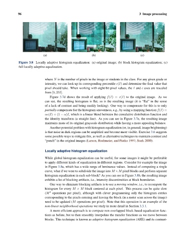
Figure 3.8 Locally adaptive histogram equalization: (a) original image; (b) block histogram equalization; (c)
full locally adaptive equalization.

where N is the number of pixels in the image or students in the class. For any given grade or
intensity, we can look up its corresponding percentile c(I) and determine the final value that
pixel should take. When working with eight-bit pixel values, the I and c axes are rescaled
from [0, 255].
Figure 3.7d shows the result of applying f(I)= c(I) to the original image. As we
can see, the resulting histogram is flat; so is the resulting image (it is “flat” in the sense
of a lack of contrast and being muddy looking). One way to compensate for this is to only
partially compensate for the histogram unevenness, e.g., by using a mapping function f(I)=
αc(I)+(1 − α)I, which is a linear blend between the cumulative distribution function and
the identity transform (a straight line). As you can see in Figure 3.7e, the resulting image
maintains more of its original grayscale distribution while having a more appealing balance.
Another potential problem with histogram equalization (or, in general, image brightening)
is that noise in dark regions can be amplified and become more visible. Exercise 3.6 suggests
some possible ways to mitigate this, as well as alternative techniques to maintain contrast and
“punch” in the original images (Larson, Rushmeier, and Piatko 1997; Stark 2000).

Locally adaptive histogram equalization

While global histogram equalization can be useful, for some images it might be preferable
to apply different kinds of equalization in different regions. Consider for example the image
in Figure 3.8a, which has a wide range of luminance values. Instead of computing a single
curve, what if we were to subdivide the image into M ×M pixel blocks and perform separate
histogram equalization in each sub-block? As you can see in Figure 3.8b, the resulting image
exhibits a lot of blocking artifacts, i.e., intensity discontinuities at block boundaries.
One way to eliminate blocking artifacts is to use a moving window, i.e., to recompute the
histogram for every M × M block centered at each pixel. This process can be quite slow
2
(M operations per pixel), although with clever programming only the histogram entries
corresponding to the pixels entering and leaving the block (in a raster scan across the image)
need to be updated (M operations per pixel). Note that this operation is an example of the
non-linear neighborhood operations we study in more detail in Section 3.3.1.
A more efficient approach is to compute non-overlapped block-based equalization func-
tions as before, but to then smoothly interpolate the transfer functions as we move between
blocks. This technique is known as adaptive histogram equalization (AHE) and its contrast-