Page 269 -

248 5 Segmentation

g(I) ׋¨

+1
׋ = 0
-1

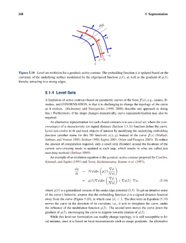
Figure 5.10 Level set evolution for a geodesic active contour. The embedding function φ is updated based on the
curvature of the underlying surface modulated by the edge/speed function g(I), as well as the gradient of g(I),
thereby attracting it to strong edges.

5.1.4 Level Sets

A limitation of active contours based on parametric curves of the form f(s), e.g., snakes, B-
snakes, and CONDENSATION, is that it is challenging to change the topology of the curve
as it evolves. (McInerney and Terzopoulos (1999, 2000) describe one approach to doing
this.) Furthermore, if the shape changes dramatically, curve reparameterization may also be
required.
An alternative representation for such closed contours is to use a level set, where the zero-
crossing(s) of a characteristic (or signed distance (Section 3.3.3)) function define the curve.
Level sets evolve to fit and track objects of interest by modifying the underlying embedding
function (another name for this 2D function) φ(x, y) instead of the curve f(s) (Malladi,
Sethian, and Vemuri 1995; Sethian 1999; Sapiro 2001; Osher and Paragios 2003). To reduce
the amount of computation required, only a small strip (frontier) around the locations of the
current zero-crossing needs to updated at each step, which results in what are called fast
marching methods (Sethian 1999).
An example of an evolution equation is the geodesic active contour proposed by Caselles,
Kimmel, and Sapiro (1997) and Yezzi, Kichenassamy, Kumar et al. (1997),

dφ ∇φ
= |∇φ|div g(I)
dt |∇φ|

∇φ
= g(I)|∇φ|div + ∇g(I) ·` φ, (5.19)
|∇φ|
where g(I) is a generalized version of the snake edge potential (5.5). To get an intuitive sense
of the curve’s behavior, assume that the embedding function φ is a signed distance function
away from the curve (Figure 5.10), in which case |φ| =1. The first term in Equation (5.19)
moves the curve in the direction of its curvature, i.e., it acts to straighten the curve, under
the influence of the modulation function g(I). The second term moves the curve down the
gradient of g(I), encouraging the curve to migrate towards minima of g(I).
While this level-set formulation can readily change topology, it is still susceptible to lo-
cal minima, since it is based on local measurements such as image gradients. An alternative