Page 267 -

246 5 Segmentation

(a) (b) (c)

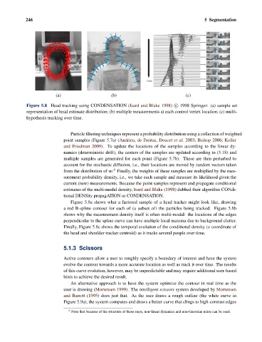
Figure 5.8 Head tracking using CONDENSATION (Isard and Blake 1998) c 1998 Springer: (a) sample set
representation of head estimate distribution; (b) multiple measurements at each control vertex location; (c) multi-
hypothesis tracking over time.

Particle filtering techniques represent a probability distribution using a collection of weighted
point samples (Figure 5.7a) (Andrieu, de Freitas, Doucet et al. 2003; Bishop 2006; Koller
and Friedman 2009). To update the locations of the samples according to the linear dy-
namics (deterministic drift), the centers of the samples are updated according to (5.18) and
multiple samples are generated for each point (Figure 5.7b). These are then perturbed to
account for the stochastic diffusion, i.e., their locations are moved by random vectors taken
6
from the distribution of w. Finally, the weights of these samples are multiplied by the mea-
surement probability density, i.e., we take each sample and measure its likelihood given the
current (new) measurements. Because the point samples represent and propagate conditional
estimates of the multi-modal density, Isard and Blake (1998) dubbed their algorithm CONdi-
tional DENSity propagATION or CONDENSATION.
Figure 5.8a shows what a factored sample of a head tracker might look like, drawing
a red B-spline contour for each of (a subset of) the particles being tracked. Figure 5.8b
shows why the measurement density itself is often multi-modal: the locations of the edges
perpendicular to the spline curve can have multiple local maxima due to background clutter.
Finally, Figure 5.8c shows the temporal evolution of the conditional density (x coordinate of
the head and shoulder tracker centroid) as it tracks several people over time.

5.1.3 Scissors

Active contours allow a user to roughly specify a boundary of interest and have the system
evolve the contour towards a more accurate location as well as track it over time. The results
of this curve evolution, however, may be unpredictable and may require additional user-based
hints to achieve the desired result.
An alternative approach is to have the system optimize the contour in real time as the
user is drawing (Mortensen 1999). The intelligent scissors system developed by Mortensen
and Barrett (1995) does just that. As the user draws a rough outline (the white curve in
Figure 5.9a), the system computes and draws a better curve that clings to high-contrast edges

6 Note that because of the structure of these steps, non-linear dynamics and non-Gaussian noise can be used.