Page 263 -

242 5 Segmentation

(a) (b)

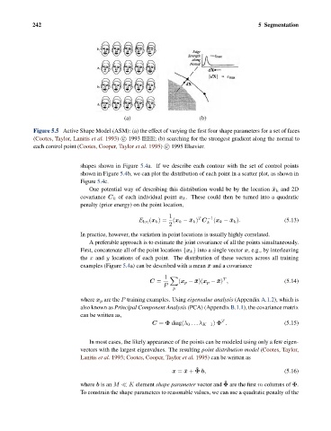
Figure 5.5 Active Shape Model (ASM): (a) the effect of varying the first four shape parameters for a set of faces
(Cootes, Taylor, Lanitis et al. 1993) c 1993 IEEE; (b) searching for the strongest gradient along the normal to
each control point (Cootes, Cooper, Taylor et al. 1995) c 1995 Elsevier.

shapes shown in Figure 5.4a. If we describe each contour with the set of control points
shown in Figure 5.4b, we can plot the distribution of each point in a scatter plot, as shown in
Figure 5.4c.
One potential way of describing this distribution would be by the location ¯x k and 2D
covariance C k of each individual point x k . These could then be turned into a quadratic
penalty (prior energy) on the point location,

1 T −1
E loc (x k )= (x k − ¯x k ) C k (x k − ¯x k ). (5.13)
2
In practice, however, the variation in point locations is usually highly correlated.
A preferable approach is to estimate the joint covariance of all the points simultaneously.
First, concatenate all of the point locations {x k } into a single vector x, e.g., by interleaving
the x and y locations of each point. The distribution of these vectors across all training
examples (Figure 5.4a) can be described with a mean ¯x and a covariance
1 T
C = (x p − ¯x)(x p − ¯x) , (5.14)
P
p
where x p are the P training examples. Using eigenvalue analysis (Appendix A.1.2), which is
also known as Principal Component Analysis (PCA) (Appendix B.1.1), the covariance matrix
can be written as,
T
C = Φ diag(λ 0 ...λ K−1 ) Φ . (5.15)

In most cases, the likely appearance of the points can be modeled using only a few eigen-
vectors with the largest eigenvalues. The resulting point distribution model (Cootes, Taylor,
Lanitis et al. 1993; Cootes, Cooper, Taylor et al. 1995) can be written as

ˆ
x = ¯x + Φ b, (5.16)
ˆ
where b is an M K element shape parameter vector and Φ are the first m columns of Φ.
To constrain the shape parameters to reasonable values, we can use a quadratic penalty of the