Page 261 -

240 5 Segmentation

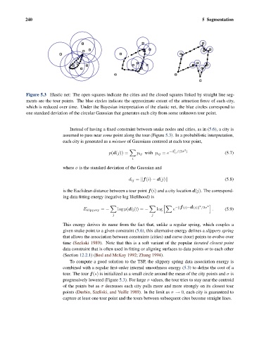
Figure 5.3 Elastic net: The open squares indicate the cities and the closed squares linked by straight line seg-
ments are the tour points. The blue circles indicate the approximate extent of the attraction force of each city,
which is reduced over time. Under the Bayesian interpretation of the elastic net, the blue circles correspond to
one standard deviation of the circular Gaussian that generates each city from some unknown tour point.

Instead of having a fixed constraint between snake nodes and cities, as in (5.6), a city is
assumed to pass near some point along the tour (Figure 5.3). In a probabilistic interpretation,
each city is generated as a mixture of Gaussians centered at each tour point,
2 2
−d ij /(2σ )
p(d(j)) = p ij with p ij = e (5.7)
i
where σ is the standard deviation of the Gaussian and

d ij = f(i) − d(j) (5.8)

is the Euclidean distance between a tour point f(i) and a city location d(j). The correspond-
ing data fitting energy (negative log likelihood) is

2 2
− f (i)−d(j) /2σ

E slippery = − log p(d(j)) = − log e . (5.9)
j j
This energy derives its name from the fact that, unlike a regular spring, which couples a
given snake point to a given constraint (5.6), this alternative energy defines a slippery spring
that allows the association between constraints (cities) and curve (tour) points to evolve over
time (Szeliski 1989). Note that this is a soft variant of the popular iterated closest point
data constraint that is often used in fitting or aligning surfaces to data points or to each other
(Section 12.2.1)(Besl and McKay 1992; Zhang 1994).
To compute a good solution to the TSP, the slippery spring data association energy is
combined with a regular first-order internal smoothness energy (5.3) to define the cost of a
tour. The tour f(s) is initialized as a small circle around the mean of the city points and σ is
progressively lowered (Figure 5.3). For large σ values, the tour tries to stay near the centroid
of the points but as σ decreases each city pulls more and more strongly on its closest tour
points (Durbin, Szeliski, and Yuille 1989). In the limit as σ → 0, each city is guaranteed to
capture at least one tour point and the tours between subsequent cites become straight lines.