Page 262 -

5.1 Active contours 241

(a) (b) (c) (d)

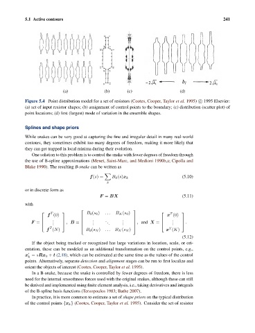
Figure 5.4 Point distribution model for a set of resistors (Cootes, Cooper, Taylor et al. 1995) c 1995 Elsevier:
(a) set of input resistor shapes; (b) assignment of control points to the boundary; (c) distribution (scatter plot) of
point locations; (d) first (largest) mode of variation in the ensemble shapes.

Splines and shape priors
While snakes can be very good at capturing the fine and irregular detail in many real-world
contours, they sometimes exhibit too many degrees of freedom, making it more likely that
they can get trapped in local minima during their evolution.
One solution to this problem is to control the snake with fewer degrees of freedom through
the use of B-spline approximations (Menet, Saint-Marc, and Medioni 1990b,a; Cipolla and
Blake 1990). The resulting B-snake can be written as

f(s)= B k (s)x k (5.10)
k
or in discrete form as
F = BX (5.11)
with
⎡ ⎤
f (0) x (0)
⎡ T ⎤ B 0 (s 0 ) ... B K (s 0 ) ⎡ T ⎤
. ⎢ . . ⎥ .
. . . . . ⎦ .
⎢ ⎥ ⎢ . ⎥ ⎢ ⎥
. ⎦ , B = ⎢ . . . ⎥ , and X = ⎣ .
F = ⎣
T
T
f (N) ⎣ B 0 (s N ) ... B K (s N ) ⎦ x (K)
(5.12)
If the object being tracked or recognized has large variations in location, scale, or ori-
entation, these can be modeled as an additional transformation on the control points, e.g.,
x = sRx k + t (2.18), which can be estimated at the same time as the values of the control

k
points. Alternatively, separate detection and alignment stages can be run to first localize and
orient the objects of interest (Cootes, Cooper, Taylor et al. 1995).
In a B-snake, because the snake is controlled by fewer degrees of freedom, there is less
need for the internal smoothness forces used with the original snakes, although these can still
be derived and implemented using finite element analysis, i.e., taking derivatives and integrals
of the B-spline basis functions (Terzopoulos 1983; Bathe 2007).
In practice, it is more common to estimate a set of shape priors on the typical distribution
of the control points {x k } (Cootes, Cooper, Taylor et al. 1995). Consider the set of resistor