Page 259 -

238 5 Segmentation

The first, originally called snakes by its inventors (Kass, Witkin, and Terzopoulos 1988)
(Section 5.1.1), is an energy-minimizing, two-dimensional spline curve that evolves (moves)
towards image features such as strong edges. The second, intelligent scissors (Mortensen
and Barrett 1995) (Section 5.1.3), allow the user to sketch in real time a curve that clings to
object boundaries. Finally, level set techniques (Section 5.1.4) evolve the curve as the zero-
set of a characteristic function, which allows them to easily change topology and incorporate
region-based statistics.
All three of these are examples of active contours (Blake and Isard 1998; Mortensen
1999), since these boundary detectors iteratively move towards their final solution under the
combination of image and optional user-guidance forces.

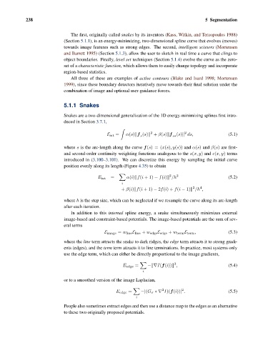
5.1.1 Snakes
Snakes are a two-dimensional generalization of the 1D energy-minimizing splines first intro-
duced in Section 3.7.1,

2
2
E int = α(s) f (s) + β(s) f (s) ds, (5.1)
s ss
where s is the arc-length along the curve f(s)=(x(s),y(s)) and α(s) and β(s) are first-
and second-order continuity weighting functions analogous to the s(x, y) and c(x, y) terms
introduced in (3.100–3.101). We can discretize this energy by sampling the initial curve
position evenly along its length (Figure 4.35) to obtain

2 2
= α(i) f(i +1) − f(i) /h (5.2)
E int
i
4
2
+ β(i) f(i +1) − 2f(i)+ f(i − 1) /h ,
where h is the step size, which can be neglected if we resample the curve along its arc-length
after each iteration.
In addition to this internal spline energy, a snake simultaneously minimizes external
image-based and constraint-based potentials. The image-based potentials are the sum of sev-
eral terms
E image = w line E line + w edge E edge + w term E term , (5.3)
where the line term attracts the snake to dark ridges, the edge term attracts it to strong gradi-
ents (edges), and the term term attracts it to line terminations. In practice, most systems only
use the edge term, which can either be directly proportional to the image gradients,

2
E edge = − ∇I(f(i)) , (5.4)
i
or to a smoothed version of the image Laplacian,

2
2
E edge = −|(G σ ∗∇ I)(f(i))| . (5.5)
i
People also sometimes extract edges and then use a distance map to the edges as an alternative
to these two originally proposed potentials.