Page 268 -

5.1 Active contours 247

(a) (b) (c)

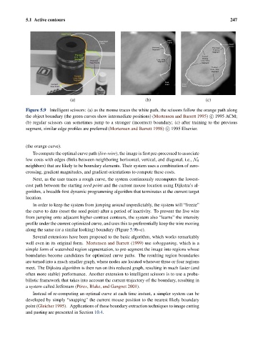
Figure 5.9 Intelligent scissors: (a) as the mouse traces the white path, the scissors follow the orange path along
the object boundary (the green curves show intermediate positions) (Mortensen and Barrett 1995) c 1995 ACM;
(b) regular scissors can sometimes jump to a stronger (incorrect) boundary; (c) after training to the previous
segment, similar edge profiles are preferred (Mortensen and Barrett 1998) c 1995 Elsevier.

(the orange curve).
To compute the optimal curve path (live-wire), the image is first pre-processed to associate
low costs with edges (links between neighboring horizontal, vertical, and diagonal, i.e., N 8
neighbors) that are likely to be boundary elements. Their system uses a combination of zero-
crossing, gradient magnitudes, and gradient orientations to compute these costs.
Next, as the user traces a rough curve, the system continuously recomputes the lowest-
cost path between the starting seed point and the current mouse location using Dijkstra’s al-
gorithm, a breadth-first dynamic programming algorithm that terminates at the current target
location.
In order to keep the system from jumping around unpredictably, the system will “freeze”
the curve to date (reset the seed point) after a period of inactivity. To prevent the live wire
from jumping onto adjacent higher-contrast contours, the system also “learns” the intensity
profile under the current optimized curve, and uses this to preferentially keep the wire moving
along the same (or a similar looking) boundary (Figure 5.9b–c).
Several extensions have been proposed to the basic algorithm, which works remarkably
well even in its original form. Mortensen and Barrett (1999) use tobogganing, which is a
simple form of watershed region segmentation, to pre-segment the image into regions whose
boundaries become candidates for optimized curve paths. The resulting region boundaries
are turned into a much smaller graph, where nodes are located wherever three or four regions
meet. The Dijkstra algorithm is then run on this reduced graph, resulting in much faster (and
often more stable) performance. Another extension to intelligent scissors is to use a proba-
bilistic framework that takes into account the current trajectory of the boundary, resulting in
a system called JetStream (P´ erez, Blake, and Gangnet 2001).
Instead of re-computing an optimal curve at each time instant, a simpler system can be
developed by simply “snapping” the current mouse position to the nearest likely boundary
point (Gleicher 1995). Applications of these boundary extraction techniques to image cutting
and pasting are presented in Section 10.4.