Page 273 -

252 5 Segmentation

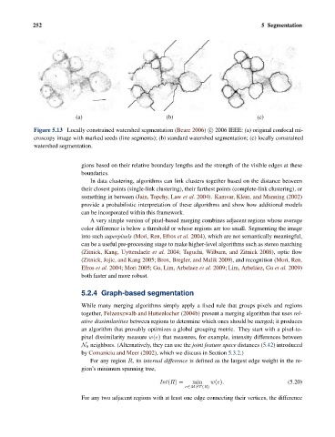
(a) (b) (c)

Figure 5.13 Locally constrained watershed segmentation (Beare 2006) c 2006 IEEE: (a) original confocal mi-
croscopy image with marked seeds (line segments); (b) standard watershed segmentation; (c) locally constrained
watershed segmentation.

gions based on their relative boundary lengths and the strength of the visible edges at these
boundaries.
In data clustering, algorithms can link clusters together based on the distance between
their closest points (single-link clustering), their farthest points (complete-link clustering), or
something in between (Jain, Topchy, Law et al. 2004). Kamvar, Klein, and Manning (2002)
provide a probabilistic interpretation of these algorithms and show how additional models
can be incorporated within this framework.
A very simple version of pixel-based merging combines adjacent regions whose average
color difference is below a threshold or whose regions are too small. Segmenting the image
into such superpixels (Mori, Ren, Efros et al. 2004), which are not semantically meaningful,
can be a useful pre-processing stage to make higher-level algorithms such as stereo matching
(Zitnick, Kang, Uyttendaele et al. 2004; Taguchi, Wilburn, and Zitnick 2008), optic flow
(Zitnick, Jojic, and Kang 2005; Brox, Bregler, and Malik 2009), and recognition (Mori, Ren,
Efros et al. 2004; Mori 2005; Gu, Lim, Arbelaez et al. 2009; Lim, Arbel´ aez, Gu et al. 2009)
both faster and more robust.

5.2.4 Graph-based segmentation

While many merging algorithms simply apply a fixed rule that groups pixels and regions
together, Felzenszwalb and Huttenlocher (2004b) present a merging algorithm that uses rel-
ative dissimilarities between regions to determine which ones should be merged; it produces
an algorithm that provably optimizes a global grouping metric. They start with a pixel-to-
pixel dissimilarity measure w(e) that measures, for example, intensity differences between
N 8 neighbors. (Alternatively, they can use the joint feature space distances (5.42) introduced
by Comaniciu and Meer (2002), which we discuss in Section 5.3.2.)
For any region R, its internal difference is defined as the largest edge weight in the re-
gion’s minimum spanning tree,
Int(R) = min w(e). (5.20)
e∈MST (R)
For any two adjacent regions with at least one edge connecting their vertices, the difference