Page 278 -

5.3 Mean shift and mode finding 257

which are the estimates of how likely a sample x i was generated from the kth Gaussian
cluster.
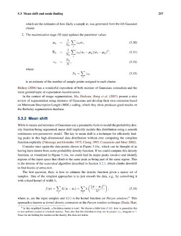
2. The maximization stage (M step) updates the parameter values
1
μ = z ik x i , (5.30)
k
N k
i
1 T
= z ik (x i − μ )(x i − μ ) , (5.31)
Σ k
k k
N k
i
N k
= , (5.32)
π k
N
where

N k = z ik . (5.33)
i
is an estimate of the number of sample points assigned to each cluster.
Bishop (2006) has a wonderful exposition of both mixture of Gaussians estimation and the
more general topic of expectation maximization.
In the context of image segmentation, Ma, Derksen, Hong et al. (2007) present a nice
review of segmentation using mixtures of Gaussians and develop their own extension based
on Minimum Description Length (MDL) coding, which they show produces good results on
the Berkeley segmentation database.

5.3.2 Mean shift

While k-means and mixtures of Gaussians use a parametric form to model the probability den-
sity function being segmented, mean shift implicitly models this distribution using a smooth
continuous non-parametric model. The key to mean shift is a technique for efficiently find-
ing peaks in this high-dimensional data distribution without ever computing the complete
function explicitly (Fukunaga and Hostetler 1975; Cheng 1995; Comaniciu and Meer 2002).
Consider once again the data points shown in Figure 5.16c, which can be thought of as
having been drawn from some probability density function. If we could compute this density
function, as visualized in Figure 5.16e, we could find its major peaks (modes) and identify
regions of the input space that climb to the same peak as being part of the same region. This
is the inverse of the watershed algorithm described in Section 5.2.1, which climbs downhill
to find basins of attraction.
The first question, then, is how to estimate the density function given a sparse set of
samples. One of the simplest approaches is to just smooth the data, e.g., by convolving it
with a fixed kernel of width h,
2

x − x i
f(x)= K(x − x i )= k , (5.34)
h 2
i i
9
where x i are the input samples and k(r) is the kernel function (or Parzen window). This
approach is known as kernel density estimation or the Parzen window technique (Duda, Hart,
9
In this simplified formula, a Euclidean metric is used. We discuss a little later (5.42) how to generalize this
to non-uniform (scaled or oriented) metrics. Note also that this distribution may not be proper, i.e., integrate to 1.
Since we are looking for maxima in the density, this does not matter.