Page 275 -

254 5 Segmentation

(a) (b) (c) (d)

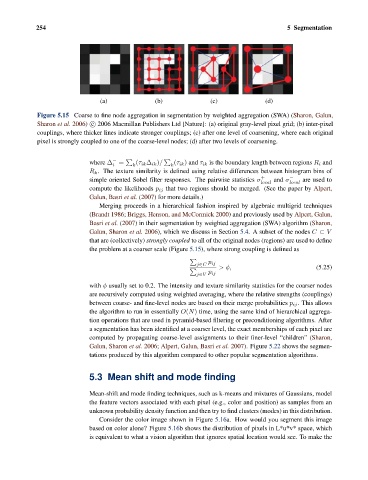
Figure 5.15 Coarse to fine node aggregation in segmentation by weighted aggregation (SWA) (Sharon, Galun,
Sharon et al. 2006) c 2006 Macmillan Publishers Ltd [Nature]: (a) original gray-level pixel grid; (b) inter-pixel
couplings, where thicker lines indicate stronger couplings; (c) after one level of coarsening, where each original
pixel is strongly coupled to one of the coarse-level nodes; (d) after two levels of coarsening.

−
where Δ = k (τ ik Δ ik )/ k (τ ik ) and τ ik is the boundary length between regions R i and
i
R k . The texture similarity is defined using relative differences between histogram bins of
simple oriented Sobel filter responses. The pairwise statistics σ + and σ − are used to
local local
compute the likelihoods p ij that two regions should be merged. (See the paper by Alpert,
Galun, Basri et al. (2007) for more details.)
Merging proceeds in a hierarchical fashion inspired by algebraic multigrid techniques
(Brandt 1986; Briggs, Henson, and McCormick 2000) and previously used by Alpert, Galun,
Basri et al. (2007) in their segmentation by weighted aggregation (SWA) algorithm (Sharon,
Galun, Sharon et al. 2006), which we discuss in Section 5.4. A subset of the nodes C ⊂ V
that are (collectively) strongly coupled to all of the original nodes (regions) are used to define
the problem at a coarser scale (Figure 5.15), where strong coupling is defined as

p ij
j∈C
>φ, (5.25)

p ij
j∈V
with φ usually set to 0.2. The intensity and texture similarity statistics for the coarser nodes
are recursively computed using weighted averaging, where the relative strengths (couplings)
between coarse- and fine-level nodes are based on their merge probabilities p ij . This allows
the algorithm to run in essentially O(N) time, using the same kind of hierarchical aggrega-
tion operations that are used in pyramid-based filtering or preconditioning algorithms. After
a segmentation has been identified at a coarser level, the exact memberships of each pixel are
computed by propagating coarse-level assignments to their finer-level “children” (Sharon,
Galun, Sharon et al. 2006; Alpert, Galun, Basri et al. 2007). Figure 5.22 shows the segmen-
tations produced by this algorithm compared to other popular segmentation algorithms.

5.3 Mean shift and mode finding

Mean-shift and mode finding techniques, such as k-means and mixtures of Gaussians, model
the feature vectors associated with each pixel (e.g., color and position) as samples from an
unknown probability density function and then try to find clusters (modes) in this distribution.
Consider the color image shown in Figure 5.16a. How would you segment this image
based on color alone? Figure 5.16b shows the distribution of pixels in L*u*v* space, which
is equivalent to what a vision algorithm that ignores spatial location would see. To make the