Page 314 -

6.3 Geometric intrinsic calibration 293

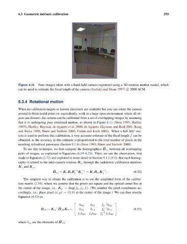
Figure 6.11 Four images taken with a hand-held camera registered using a 3D rotation motion model, which
can be used to estimate the focal length of the camera (Szeliski and Shum 1997) c 2000 ACM.

6.3.4 Rotational motion

When no calibration targets or known structures are available but you can rotate the camera
around its front nodal point (or, equivalently, work in a large open environment where all ob-
jects are distant), the camera can be calibrated from a set of overlapping images by assuming
that it is undergoing pure rotational motion, as shown in Figure 6.11 (Stein 1995; Hartley
1997b; Hartley, Hayman, de Agapito et al. 2000; de Agapito, Hayman, and Reid 2001; Kang
◦
and Weiss 1999; Shum and Szeliski 2000; Frahm and Koch 2003). When a full 360 mo-
tion is used to perform this calibration, a very accurate estimate of the focal length f can be
obtained, as the accuracy in this estimate is proportional to the total number of pixels in the
resulting cylindrical panorama (Section 9.1.6)(Stein 1995; Shum and Szeliski 2000).
˜
To use this technique, we first compute the homographies H ij between all overlapping
pairs of images, as explained in Equations (6.19–6.23). Then, we use the observation, first
made in Equation (2.72) and explored in more detail in Section 9.1.3 (9.5), that each homog-
raphy is related to the inter-camera rotation R ij through the (unknown) calibration matrices
K i and K j ,
˜ −1 −1 −1
H ij = K i R i R j K j = K i R ij K j . (6.52)

The simplest way to obtain the calibration is to use the simplified form of the calibra-
tion matrix (2.59), where we assume that the pixels are square and the optical center lies at
the center of the image, i.e., K k = diag(f k ,f k , 1). (We number the pixel coordinates ac-
cordingly, i.e., place pixel (x, y)=(0, 0) at the center of the image.) We can then rewrite
Equation (6.52)as

⎡ −1 ⎤
h 00 h 01 f 0 h 02
−1 ˜ −1
R 10 ∼ K H 10 K 0 ∼ ⎣ f ⎦ , (6.53)
1 h 10 h 11 0 h 12
f −1
f 1 h 20 f 1 h 21 f 1 h 22
0
˜
where h ij are the elements of H 10 .