Page 312 -

6.3 Geometric intrinsic calibration 291

x 1 x 0 x 1 x 0
c

x 2 x 2

(a) (b)
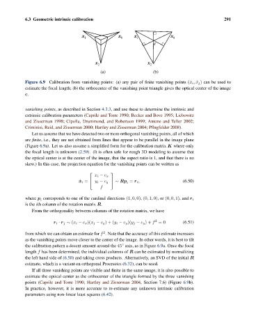
Figure 6.9 Calibration from vanishing points: (a) any pair of finite vanishing points (ˆx i , ˆx j ) can be used to
estimate the focal length; (b) the orthocenter of the vanishing point triangle gives the optical center of the image
c.

vanishing points, as described in Section 4.3.3, and use these to determine the intrinsic and
extrinsic calibration parameters (Caprile and Torre 1990; Becker and Bove 1995; Liebowitz
and Zisserman 1998; Cipolla, Drummond, and Robertson 1999; Antone and Teller 2002;
Criminisi, Reid, and Zisserman 2000; Hartley and Zisserman 2004; Pflugfelder 2008).
Let us assume that we have detected two or more orthogonal vanishing points, all of which
are finite, i.e., they are not obtained from lines that appear to be parallel in the image plane
(Figure 6.9a). Let us also assume a simplified form for the calibration matrix K where only
the focal length is unknown (2.59). (It is often safe for rough 3D modeling to assume that
the optical center is at the center of the image, that the aspect ratio is 1, and that there is no
skew.) In this case, the projection equation for the vanishing points can be written as

⎡ ⎤
x i − c x
ˆ x i = ⎣ y i − c y ⎦ ∼ Rp = r i , (6.50)
i
f
where p corresponds to one of the cardinal directions (1, 0, 0), (0, 1, 0),or (0, 0, 1), and r i
i
is the ith column of the rotation matrix R.
From the orthogonality between columns of the rotation matrix, we have

2
r i · r j ∼ (x i − c x )(x j − c y )+(y i − c y )(y j − c y )+ f =0 (6.51)
2
from which we can obtain an estimate for f . Note that the accuracy of this estimate increases
as the vanishing points move closer to the center of the image. In other words, it is best to tilt
the calibration pattern a decent amount around the 45 axis, as in Figure 6.9a. Once the focal
◦
length f has been determined, the individual columns of R can be estimated by normalizing
the left hand side of (6.50) and taking cross products. Alternatively, an SVD of the initial R
estimate, which is a variant on orthogonal Procrustes (6.32), can be used.
If all three vanishing points are visible and finite in the same image, it is also possible to
estimate the optical center as the orthocenter of the triangle formed by the three vanishing
points (Caprile and Torre 1990; Hartley and Zisserman 2004, Section 7.6) (Figure 6.9b).
In practice, however, it is more accurate to re-estimate any unknown intrinsic calibration
parameters using non-linear least squares (6.42).