Page 61 - Control Theory in Biomedical Engineering

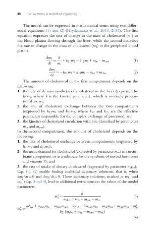
48 Control theory in biomedical engineering

The model can be expressed in mathematical terms using two differ-
ential equations: (1) and (2) (Hrydziuszko et al., 2014, 2015). The first
equation expresses the rate of change in the mass of cholesterol (m 1 )in
the blood plasma flowing through the liver, while the second describes
therateofchangeinthe mass of cholesterol(m 2 ) in the peripheral blood
plasma.

k
dm 1
¼ + k 21 m 2 k 12 m 1 + m in m out (1)
dt m 1
dm 2
¼ k 21 m 2 + k 12 m 1 m tis + m diet (2)
dt
The amount of cholesterol in the first compartment depends on the
following:
1. therateof de novo synthesis of cholesterol in the liver (expressed by
k/m 1 ,where k is the kinetic parameter), which is inversely propor-
tional to m 1 ;
2. the rate of cholesterol exchange between the two compartments
(expressed by k 12 m 1 and k 21 m 2 , where k 12 and k 21 are the effective
parameters responsible for the complex exchange of processes); and
3. the kinetics of cholesterol circulation with bile (described by parameters
m in and m out ).
In the second compartment, the amount of cholesterol depends on the
following:
1. the rate of cholesterol exchange between compartments (expressed by
k 12 m 1 and k 21 m 2 );
2. the tissue demand for cholesterol (expressed by parameter m tis ) as a mem-
brane component or as a substrate for the synthesis of steroid hormones
and vitamin D; and
3. the rate of intake of dietary cholesterol (expressed by parameter m diet ).
Eqs. (1), (2) enable finding analytical stationary solutions, that is, when
*
dm 1 /dt¼0 and dm 2 /dt¼0. These stationary solutions, marked as m 1 and
*
m 2 (Eqs. 3 and 4), lead to additional restrictions on the values of the model
parameters.
k
∗
m ¼ (3)
1
m diet + m in m out m tis
m 2 + m diet m in m diet m out kk 12 2m diet m tis m in m tis + m out m tis + m 2
∗ diet tis
m ¼
2
k 21 m diet + m in m out m tis Þ
ð
(4)