Page 62 - Control Theory in Biomedical Engineering

Mathematical modeling of cholesterol homeostasis 49

Because the mass must be positive, Eq. (3) leads to the following
relationship: m diet +m in >m out +m tis . Similarly, Eq. (4) requires that
+m diet m in m diet m out k k 12 2 m diet m tis m in m tis +m out m tis +>0 be-
cause k 21 (m diet +m in m out m tis ) is greater than 0, which results from fur-
ther analysis of the model solutions.
* *
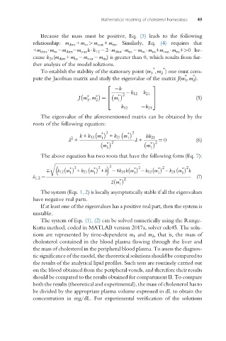
To establish the stability of the stationary point (m 1 ,m 2 ) one must com-
* *
pute the Jacobian matrix and study the eigenvalue of the matrix J(m 1 ,m 2 ).
k
2 3
k 12 k 21
* 2
∗
Jm , m ∗ 6 m 7 (5)
1 2 ¼ 4 1 5
k 12 k 21
The eigenvalue of the aforementioned matrix can be obtained by the
roots of the following equation:

* 2 * 2
k + k 12 m 1 + k 21 m 1 kk 21
2
λ + ¼ 0 (6)
* 2 λ + * 2
m 1 m 1
The above equation has two roots that have the following form (Eq. 7):
r ffiffiffiffiffiffiffiffiffiffiffiffiffiffiffiffiffiffiffiffiffiffiffiffiffiffiffiffiffiffiffiffiffiffiffiffiffiffiffiffiffiffiffiffiffiffiffiffiffiffiffiffiffiffiffiffiffiffiffiffiffiffiffiffiffiffiffiffiffiffiffiffiffiffiffiffiffiffiffiffi
2
* 2 * 2 * 2 * 2 * 2
k 12 m + k 21 m + k 4k 21 km k 12 m k 21 m k
1 1 1 1 1
λ 1,2 ¼ (7)
* 2
2 m
1
The system (Eqs. 1, 2) is locally asymptotically stable if all the eigenvalues
have negative real parts.
If at least one of the eigenvalues has a positive real part, then the system is
unstable.
The system of Eqs. (1), (2) can be solved numerically using the Runge-
Kutta method, coded in MATLAB version 2017a, solver ode45. The solu-
tions are represented by time-dependent m 1 and m 2 , that is, the mass of
cholesterol contained in the blood plasma flowing through the liver and
the mass of cholesterol in the peripheral blood plasma. To assess the diagnos-
tic significance of the model, the theoretical solutions should be compared to
the results of the analytical lipid profiles. Such tests are routinely carried out
on the blood obtained from the peripheral vessels, and therefore their results
should be compared to the results obtained for compartment II. To compare
both the results (theoretical and experimental), the mass of cholesterol has to
be divided by the appropriate plasma volume expressed in dL to obtain the
concentration in mg/dL. For experimental verification of the solutions