Page 254 - DSP Integrated Circuits

6.5 DIFFERENCE EQUATIONS 239

If a node value (for example, u\) is computed earlier than needed, an auxiliary
node must be introduced. The branch connecting the nodes represents storing the
value in memory. The sample interval is assumed here to begin with execution of
the leftmost operations and end with the computation of the nodes belonging to set
NI. Once the latter have been computed, the computations belonging to the next
sample interval can begin. In fact, the nodes in sets NI and Ny can be regarded as
belonging to the same node set. Six time steps are required to complete the opera-
tions within one sample interval.
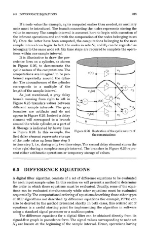
It is illustrative to draw the pre-
cedence form on a cylinder, as shown
in Figure 6.26, to demonstrate the
cyclic nature of the computations. The
computations are imagined to be per-
formed repeatedly around the cylin-
der. The circumference of the cylinder
corresponds to a multiple of the
length of the sample interval.
As just mentioned, a gray delay
branch running from right to left in
Figure 6.25 transfers values between
different sample intervals. The gray
branches are artifacts and do not
appear in Figure 6.26. Instead a delay
element will correspond to a branch
around the whole cylinder, or a part of
it. Storage is indicated by heavy lines
in Figure 6.26. In this example, the Figure 6.26 llustration of the cyclic nature of
a . j -, -, , , . the computations
first delay element represents storage
of the node value UQ from time step 5
to time step 1, i.e., during only two time steps. The second delay element stores the
value VI(H) during a complete sample interval. The branches in Figure 6.26 repre-
sent either arithmetic operations or temporary storage of values.

6.5 DIFFERENCE EQUATIONS

A digital filter algorithm consists of a set of difference equations to be evaluated
for each input sample value. In this section we will present a method to determine
the order in which these equations must be evaluated. Usually, some of the equa-
tions can be evaluated simultaneously while other equations must be evaluated
sequentially. The computational ordering of equations describing those other types
of DSP algorithms not described by difference equations (for example, FFTs) can
also be derived by the method presented shortly. In both cases, this ordered set of
equations is a useful starting point for implementing the algorithm in software
using a standard signal processor or a multicomputer.
The difference equations for a digital filter can be obtained directly from its
signal-flow graph in precedence form. The signal values corresponding to node set
NI are known at the beginning of the sample interval. Hence, operations having