Page 107 -

HAN 09-ch02-039-082-9780123814791

70 Chapter 2 Getting to Know Your Data 2011/6/1 3:15 Page 70 #32

Alternatively, similarity can be computed as
m
sim(i, j) = 1 − d(i, j) = . (2.12)
p
Proximity between objects described by nominal attributes can be computed using
an alternative encoding scheme. Nominal attributes can be encoded using asymmetric
binary attributes by creating a new binary attribute for each of the M states. For an
object with a given state value, the binary attribute representing that state is set to 1,
while the remaining binary attributes are set to 0. For example, to encode the nominal
attribute map color, a binary attribute can be created for each of the five colors previ-
ously listed. For an object having the color yellow, the yellow attribute is set to 1, while
the remaining four attributes are set to 0. Proximity measures for this form of encoding
can be calculated using the methods discussed in the next subsection.

2.4.3 Proximity Measures for Binary Attributes
Let’s look at dissimilarity and similarity measures for objects described by either
symmetric or asymmetric binary attributes.
Recall that a binary attribute has only one of two states: 0 and 1, where 0 means that
the attribute is absent, and 1 means that it is present (Section 2.1.3). Given the attribute
smoker describing a patient, for instance, 1 indicates that the patient smokes, while 0
indicates that the patient does not. Treating binary attributes as if they are numeric can
be misleading. Therefore, methods specific to binary data are necessary for computing
dissimilarity.
“So, how can we compute the dissimilarity between two binary attributes?” One
approach involves computing a dissimilarity matrix from the given binary data. If all
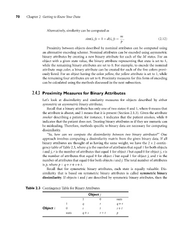
binary attributes are thought of as having the same weight, we have the 2 × 2 contin-
gency table of Table 2.3, where q is the number of attributes that equal 1 for both objects
i and j, r is the number of attributes that equal 1 for object i but equal 0 for object j, s is
the number of attributes that equal 0 for object i but equal 1 for object j, and t is the
number of attributes that equal 0 for both objects i and j. The total number of attributes
is p, where p = q + r + s + t.
Recall that for symmetric binary attributes, each state is equally valuable. Dis-
similarity that is based on symmetric binary attributes is called symmetric binary
dissimilarity. If objects i and j are described by symmetric binary attributes, then the

Table 2.3 Contingency Table for Binary Attributes
Object j
1 0 sum
1 q r q + r
Object i 0 s t s + t
sum q + s r + t p