Page 104 -
P. 104
Page 67
3:15
2011/6/1
#29
HAN 09-ch02-039-082-9780123814791
2.4 Measuring Data Similarity and Dissimilarity 67
This section presents similarity and dissimilarity measures, which are referred to as
measures of proximity. Similarity and dissimilarity are related. A similarity measure for
two objects, i and j, will typically return the value 0 if the objects are unalike. The higher
the similarity value, the greater the similarity between objects. (Typically, a value of 1
indicates complete similarity, that is, the objects are identical.) A dissimilarity measure
works the opposite way. It returns a value of 0 if the objects are the same (and therefore,
far from being dissimilar). The higher the dissimilarity value, the more dissimilar the
two objects are.
In Section 2.4.1 we present two data structures that are commonly used in the
above types of applications: the data matrix (used to store the data objects) and the
dissimilarity matrix (used to store dissimilarity values for pairs of objects). We also
switch to a different notation for data objects than previously used in this chapter
since now we are dealing with objects described by more than one attribute. We then
discuss how object dissimilarity can be computed for objects described by nominal
attributes (Section 2.4.2), by binary attributes (Section 2.4.3), by numeric attributes
(Section 2.4.4), by ordinal attributes (Section 2.4.5), or by combinations of these
attribute types (Section 2.4.6). Section 2.4.7 provides similarity measures for very long
and sparse data vectors, such as term-frequency vectors representing documents in
information retrieval. Knowing how to compute dissimilarity is useful in studying
attributes and will also be referenced in later topics on clustering (Chapters 10 and 11),
outlier analysis (Chapter 12), and nearest-neighbor classification (Chapter 9).
2.4.1 Data Matrix versus Dissimilarity Matrix
In Section 2.2, we looked at ways of studying the central tendency, dispersion, and spread
of observed values for some attribute X. Our objects there were one-dimensional, that
is, described by a single attribute. In this section, we talk about objects described by mul-
tiple attributes. Therefore, we need a change in notation. Suppose that we have n objects
(e.g., persons, items, or courses) described by p attributes (also called measurements or
features, such as age, height, weight, or gender). The objects are x 1 = (x 11 ,x 12 ,...,x 1p ),
x 2 = (x 21 ,x 22 ,...,x 2p ), and so on, where x ij is the value for object x i of the jth attribute.
For brevity, we hereafter refer to object x i as object i. The objects may be tuples in a
relational database, and are also referred to as data samples or feature vectors.
Main memory-based clustering and nearest-neighbor algorithms typically operate
on either of the following two data structures:
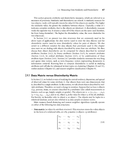
Data matrix (or object-by-attribute structure): This structure stores the n data objects
in the form of a relational table, or n-by-p matrix (n objects ×p attributes):
x 11 ··· x 1f ··· x 1p
··· ··· ··· ··· ···
x i1 ··· x if ··· x ip . (2.8)
··· ··· ··· ··· ···
x n1 ··· x nf ··· x np

