Page 174 -

3:17 Page 137
2011/6/1
HAN
#13
11-ch04-125-186-9780123814791
4.2 Data Warehouse Modeling: Data Cube and OLAP 137

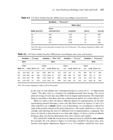
Table 4.2 2-D View of Sales Data for AllElectronics According to time and item

location = “Vancouver”
item (type)
home
time (quarter) entertainment computer phone security
Q1 605 825 14 400
Q2 680 952 31 512
Q3 812 1023 30 501
Q4 927 1038 38 580

Note: The sales are from branches located in the city of Vancouver. The measure displayed is dollars sold
(in thousands).

Table 4.3 3-D View of Sales Data for AllElectronics According to time, item, and location
location = “Chicago” location = “New York” location = “Toronto” location = “Vancouver”
item item item item

home home home home
time ent. comp. phone sec. ent. comp. phone sec. ent. comp. phone sec. ent. comp. phone sec.

Q1 854 882 89 623 1087 968 38 872 818 746 43 591 605 825 14 400
Q2 943 890 64 698 1130 1024 41 925 894 769 52 682 680 952 31 512
Q3 1032 924 59 789 1034 1048 45 1002 940 795 58 728 812 1023 30 501
Q4 1129 992 63 870 1142 1091 54 984 978 864 59 784 927 1038 38 580
Note: The measure displayed is dollars sold (in thousands).

in this way, we may display any n-dimensional data as a series of (n − 1)-dimensional
“cubes.” The data cube is a metaphor for multidimensional data storage. The actual
physical storage of such data may differ from its logical representation. The important
thing to remember is that data cubes are n-dimensional and do not confine data to 3-D.
Tables 4.2 and 4.3 show the data at different degrees of summarization. In the data
warehousing research literature, a data cube like those shown in Figures 4.3 and 4.4 is
often referred to as a cuboid. Given a set of dimensions, we can generate a cuboid for
each of the possible subsets of the given dimensions. The result would form a lattice of
cuboids, each showing the data at a different level of summarization, or group-by. The
lattice of cuboids is then referred to as a data cube. Figure 4.5 shows a lattice of cuboids
forming a data cube for the dimensions time, item, location, and supplier.
The cuboid that holds the lowest level of summarization is called the base cuboid.
For example, the 4-D cuboid in Figure 4.4 is the base cuboid for the given time, item,
location, and supplier dimensions. Figure 4.3 is a 3-D (nonbase) cuboid for time, item,