Page 196 - Decision Making Applications in Modern Power Systems

Adaptive estimation and tracking of power quality disturbances Chapter | 6 159

6.2.2.2 Recursive least square algorithm
RLS filtering algorithm is based on matrix inversion lemma. The rate of conver-
gence of this filter is typically much faster than the LMS algorithm due to the fact
that input data is whitened by using the inverse correlation matrix of the data,
assumed to be of zero mean. But RLS is computationally more complex than LMS.
A weighting factor is introduced to the definition of ξðnÞ as
n
X
2
ξðnÞ 5 βðn; iÞ eðiÞ ð6:24Þ

i51
where eðiÞ is the difference between the desired response, dðiÞ, and the out-
put, yðiÞ
H
eðiÞ 5 dðiÞ 2 yðiÞ 5 dðiÞ 2 w ðnÞuðiÞ ð6:25Þ
where uðiÞ is the tap input vector at time i, defined by
T
uðiÞ 5 ½uðiÞ; uði21Þ; ...; uði2M11ފ ð6:26Þ
and wðnÞ is the tap weight vector at time n, defined by

wðnÞ 5 ½ω 0 ðnÞ; ω 1 ðnÞ; ...; ω M21 ðnފ ð6:27Þ
The algorithm estimates iteratively by initializing weight vector and esti-
mation covariance to zero.
21
^ wð0Þ 5 0 ; Pð0Þ 5 δ I ð6:28Þ
and δ is the small positive constant for high SNR and the large positive con-
stant for low SNR.
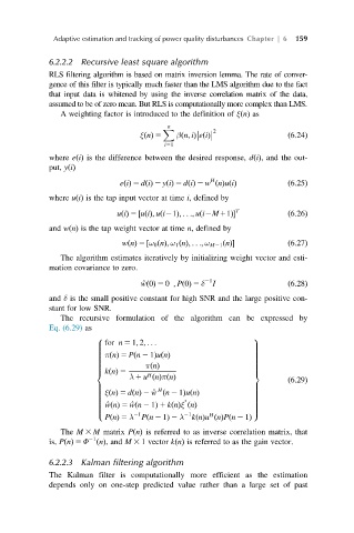
The recursive formulation of the algorithm can be expressed by
Eq. (6.29) as
for n 5 1; 2; ...
8 9
> >
> >
> >
> >
πðnÞ 5 Pðn 2 1ÞuðnÞ
> >
> >
> >
> >
> πðnÞ >
> >
> kðnÞ 5 >
< H =
λ 1 u ðnÞπðnÞ
ð6:29Þ
> >
> H >
ξðnÞ 5 dðnÞ 2 ^ w ðn 2 1ÞuðnÞ
> >
> >
> >
> >

> >
^ wðnÞ 5 ^ wðn 2 1Þ 1 kðnÞξ ðnÞ
> >
> >
> >
> >
: 21 21 H ;
PðnÞ 5 λ Pðn 2 1Þ 2 λ kðnÞu ðnÞPðn 2 1Þ
The M 3 M matrix PðnÞ is referred to as inverse correlation matrix, that
21
is, PðnÞ 5 Φ ðnÞ, and M 3 1 vector kðnÞ is referred to as the gain vector.
6.2.2.3 Kalman filtering algorithm
The Kalman filter is computationally more efficient as the estimation
depends only on one-step predicted value rather than a large set of past