Page 429 - Design and Operation of Heat Exchangers and their Networks

412 Design and operation of heat exchangers and their networks

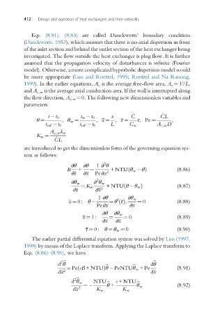
Eqs. (8.81), (8.83) are called Danckwerts’ boundary condition
(Danckwerts, 1953), which assumes that there is no axial dispersion in front
of the inlet section and behind the outlet section of the heat exchanger being
investigated. The flow outside the heat exchanger is plug flow. It is further
assumed that the propagation velocity of disturbances is infinite (Fourier
model). Otherwise, a more complicated hyperbolic dispersion model would
be more appropriate (Luo and Roetzel, 1995; Roetzel and Na Ranong,
1999). In the earlier equations, A c is the average free-flow area, A c ¼V/L,
and A c,w is the average axial conduction area. If the wall is interrupted along
the flow direction, A c,w ¼0. The following new dimensionless variables and
parameters
_
t t 0 t w t 0 x C _ CL
θ ¼ , θ w ¼ , x ¼ , τ ¼ τ,Pe ¼ ,
t ref t 0 t ref t 0 L C w A c,w D
A c,w λ w
K w ¼
_
CL
are introduced to get the dimensionless form of the governing equation sys-
tem as follows:
∂θ ∂θ 1 ∂ θ
2
B + ¼ + NTU θ w θÞ (8.86)
ð
∂τ ∂x Pe∂x 2
2
∂θ w ∂ θ w + NTU θ θ w Þ (8.87)
ð
∂τ ¼ K w ∂x 2
1 ∂θ ∂θ w
0
x ¼ 0 : θ ¼ θ τðÞ, ¼ 0 (8.88)
Pe∂x ∂x
∂θ ∂θ w
x ¼ 1 : ¼ ¼ 0 (8.89)
∂x ∂x
τ ¼ 0 : θ ¼ θ w ¼ 0 (8.90)

The earlier partial differential equation system was solved by Luo (1997,
1998) by means of the Laplace transform. Applying the Laplace transform to
Eqs. (8.86)–(8.90), we have
d θ dθ
2 e
e
¼ Pe sB + NTUÞθ PeNTUθ w +Pe (8.91)
e
e
ð
dx 2 dx
2 e
d θ w NTU s + NTU
θ +
¼ e e (8.92)
θ w
dx 2 K w K w