Page 562 - Design and Operation of Heat Exchangers and their Networks

Appendix 545

fprintf(ID, 'h_f_h =%f, h_f_c =%f, delta_f_h =%f, delta_f_c =%f, ', ...
h_f_h, h_f_c, delta_f_h, delta_f_c);
fprintf(ID, 'l_s_h =%f, l_s_c =%f, FPM_h =%f, FPM_c%f, Q =%f\n', ...
l_s_h, l_s_c, FPM_h, FPM_c, Q_cal);
fprintf(ID, 'x = [');

for i=1: nvars
fprintf('%f ', x(i) ∗ scale(i));
fprintf(ID, '%f ', x(i) ∗ scale(i));
end
fprintf(']\n');
fprintf(ID, ']\n');
fclose(ID);
end
end

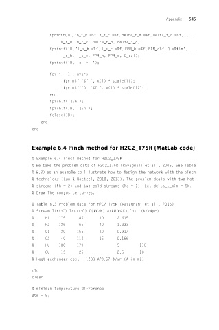
Example 6.4 Pinch method for H2C2_175R (MatLab code)
% Example 6.4 Pinch method for H2C2_175R
% We take the problem data of H2C2_175R (Ravagnani et al., 2005. See Table
% 6.3) as an example to illustrate how to design the network with the pinch
% technology (Luo & Roetzel, 2010, 2013). The problem deals with two hot
% streams (Nh = 2) and two cold streams (Nc = 2). Let delta_t_min = 5K.
% Draw The composite curves.

% Table 6.3 Problem data for H2C2_175R (Ravagnani et al., 2005)
% Stream Tin(°C) Tout(°C) C(kW/K) a(kW/m2K) Cost ($/kWyr)
% H1 175 45 10 2.615
% H2 125 65 40 1.333
% C1 20 155 20 0.917
% C2 40 112 15 0.166
% HU 180 179 5 110
% CU 15 25 2.5 10
% Heat exchanger cost = 1200 A 0.57 $/yr (A in m2)
^
clc
clear
% minimum temperature difference
dtm = 5;