Page 62 - Design and Operation of Heat Exchangers and their Networks

Basic thermal design theory for heat exchangers 49

For practical design and rating purposes, the model with two variable
parameters, Pe and Ma, is not well suited. For that reason, the unity Mach
number dispersion model has been developed in which the fixed mean value
Ma¼1 is applied together with the dispersive Peclet number (Roetzel,
2010; Roetzel et al., 2011; Na Ranong and Roetzel, 2012; Roetzel and
Na Ranong, 2014, 2015, 2018a). The main advantage of this model over
the parabolic model is that it leads merely to simple corrections of the mean
temperature difference or the heat transfer coefficients, while the known
steady-state design and rating methods can further be applied by using the
true mean temperature difference for dispersive flow Δt m,d together with
the true overall heat transfer coefficient in Eq. (2.68) as

Q ¼ kAΔt m,d (2.108)
or the hypothetic mean temperature difference Δt m (the mean temperature
difference in an equivalent nondispersive plug-flow heat exchanger) and the
∗
apparent overall heat transfer coefficient k as
∗
Q ¼ k AΔt m (2.109)
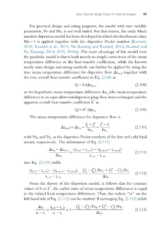
The mean temperature difference for dispersive flow is
t t 00 t t 0
00
0
Δt m,d ¼ Δt m h h c c (2.110)
Pe h Pe c
with Pe h and Pe c as the dispersive Peclet numbers of the hot and cold fluid
stream, respectively. The substitution of Eq. (2.111)

ð
Δt m Δt m,d ð t h,m t c,m Þ t h,m,d t c,m,d Þ
¼ (2.111)
Δt m t h,m t c,m
into Eq. (2.110) yields

0 00 00 0
ð t h,m t c,m Þ t h,m,d t c,m,d Þ t t =Pe h + t t =Pe c
ð
c
h
h
c
¼ (2.112)
t h,m t c,m Δt m
From the theory of the dispersion model, it follows that for constant
∗
values of k or k , the earlier ratio of mean temperature differences is equal
to the related local temperature differences. Thus, the indices “m” on the
left-hand side of Eq. (2.112) can be omitted. Rearranging Eq. (2.112) yields

0 00 00 0
Δt d t h,d t c,d t t =Pe h + t t =Pe c
c
h
h
c
¼ ¼ 1 (2.113)
t h t c t h t c Δt m