Page 594 - Design for Six Sigma a Roadmap for Product Development

550 Chapter Fifteen

k
m
^
^
^ 2 1

(y ij β 0 β 1 M j ) 2 (15.5)
MSE
mk 2 j 1 i 1
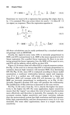
Sometimes we want to fit a regression line passing the origin; that is,
ß 0 0 is assumed. This case arises where we need y 0, when M 0
(no signal, no response). Then the regression equation is
^
y β 1 M ε (15.6)
k m

M j y ij
^ j 1i 1
β (15.7)
k
1
m
M j 2
j 1
m
k
^
^ 2 1

(y ij β 1 M j ) 2 (15.8)
MSE
mk 1 j 1 i 1
All these calculations can be easily performed by a standard statisti-
cal package such as MINITAB.
Clearly, the signal-to-noise ratio (S/N) is inversely proportional to
MSE, and S/N is proportional to β 1 . MSE is the mean squared error for
linear regression. For a perfect linear regression fit, there is no scat-
tering around the linear regression line, the MSE will be equal to zero,
and S/N will be infinity, which will be an ideal S/N.
Figure 15.10 shows what will affect S/N in a signal-response system.
For Fig. 15.10a and b it is obvious that S/N is inversely proportional to
variation, because high variation will increase MSE, thus decreasing
S/N. For Fig. 15.10c, since S/N is evaluated according to linear model
assumption, a nonlinear relationship between signal and response,
even if it is a perfect one, will create residuals for a linear fit.
Therefore, MSE will increase while S/N will decrease (i.e., S/N and
MSE are inversely proportional to nonlinearity, as in Fig. 15.10c).
Actually, Taguchi’s dynamic S/N ratio will penalize the nonlinearity.
The justification of this criterion is discussed in the next section.
For Fig. 15.10e and f, from Eq. (15.1), clearly the higher the sensi-
tivity b, the higher the S/N. For some application, higher sensitivity
means that the “signal” can adjust the level of main transformation
more effectively and therefore is desirable. For example, for a mea-
surement system, higher sensitivity and lower variation indicate
that the measurement system has high resolution and high repeata-
bility, high reproducibility, and low measurement error; so it is very
desirable. For some other applications, there is a target value for
sensitivity.