Page 142 - Design of Solar Thermal Power Plants

3.2 HELIOSTAT FIELD EFFICIENCY ANALYSIS 127

FIGURE 3.3 cont’d.

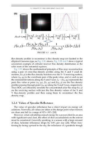
flux-density profiles to reconstruct a flux density map not limited to the
elliptical Gaussian type, as Fig. 3.3G shows. Fig. 3.3E and F show a typical
calculation example of cylinder receiver flux density distribution at the
solar noon of the autumnal equinox.
Fig. 3.3F shows the mathematical principle of flux map reconstruction
using a pair of cross-flux-density profiles along the X and Y axial di-
rections. f(x, y) is the flux density function over the XeY receiving surface,
where (x 0 , y 0 ) is the coordinate pair of the peak value, and sx and sy are
the standard deviations along the X and Yaxes. I 0 ¼ f(x 0 , y 0 ) represents the
peak flux value at point (x 0 , y 0 ). f(x, y 0 ) and f(x 0 , y) are the flux density
profiles passing through point (x 0 , y 0 ) along the X and Yaxes, respectively.
Thus HOC can efficiently simulate the concentrated solar flux map f(x, y)
on the receiving surface with just the flux density values of the X and
Y flux-density profiles and then using them to reconstruct the flux
density map.

3.2.4 Values of Specular Reflectance
The value of specular reflectance has a direct impact on energy cal-
culations. Normally, all values are taken at the design point when mirrors
are clean and fall in a range of 92%e94% [20].
However, when calculating annual energy for a power plant in an area
with significant sand dust, the effect of dust accumulation on the mirror
must be considered. Generally speaking, in a season with a large amount
of dust, heliostat reflectance drops by 0.8% per day [20]. When func-
tioning by facing upward to the sky, the reflectance of a parabolic trough