Page 49 - Determinants and Their Applications in Mathematical Physics

34 3. Intermediate Determinant Theory

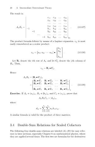
The result is:
...
c 11 c 12
c 1n
...
c 21 c 22
c 2n
... ... ...

...

c n1 c n2
... c nn . (3.3.17)
−1 b 11 b 12 ... b 1n
A n B n =
−1 ...

b 21 b 22 b 2n
... ... ... ...

...
−1 b n1 b n2 ... b nn 2n

The product formula follows by means of a Laplace expansion. c ij is most
easily remembered as a scalar product:
 b 1j 

 . (3.3.18)
 b 2j 
c ij = a i1 a i2 ··· a in • 
···
b nj
Let R i denote the ith row of A n and let C j denote the jth column of
B n . Then,
c ij = R i • C j .
Hence
A n B n = |R i • C j | n

R 1 • C 1 R 1 • C 2 ··· R 1 • C n

R 2 • C 1 R 2 • C 2 ··· R 2 • C n
. (3.3.19)
=
······ ······ ··· ······

R n • C 1 R n • C 2 ··· R n • C n n
Exercise. If A n = |a ij | n , B n = |b ij | n , and C n = |c ij | n , prove that
A n B n C n = |d ij | n ,
where
n n

d ij = a ir b rs c sj .
r=1 s=1
A similar formula is valid for the product of three matrices.

3.4 Double-Sum Relations for Scaled Cofactors

The following four double-sum relations are labeled (A)–(D) for easy refer-
ence in later sections, especially Chapter 6 on mathematical physics, where
they are applied several times. The first two are formulas for the derivatives