Page 63 - Determinants and Their Applications in Mathematical Physics

48 3. Intermediate Determinant Theory
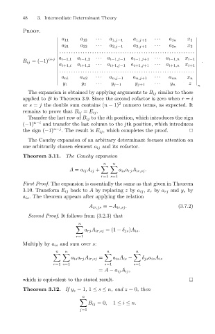
Proof.

a 11 a 12 ··· a 1,j−1 a 1,j+1 ··· a 1n x 1

a 21 a 22 ··· a 2,j−1 a 2,j+1 ··· a 2n x 2

..........................................................

B ij =(−1) i+j a i−1,1 a i−1,2 ··· a i−1,j−1 a i−1,j+1 ··· a i−1,n x i−1 .

a i+1,2 ··· a i+1,j−1 a i+1,j+1 ··· a i+1,n x i+1
a i+1,i

..........................................................

a n1 a n2 ··· a n,j−1 a n,j+1 ··· a nn x n

y 1 y 2 ··· y j−1 y j+1 ··· z
y n
n
The expansion is obtained by applying arguments to B ij similar to those
applied to B in Theorem 3.9. Since the second cofactor is zero when r = i
2
or s = j the double sum contains (n − 1) nonzero terms, as expected. It
remains to prove that B ij = E ij .
Transfer the last row of B ij to the ith position, which introduces the sign
(−1) n−i and transfer the last column to the jth position, which introduces
the sign (−1) n−j . The result is E ij , which completes the proof.
The Cauchy expansion of an arbitrary determinant focuses attention on
one arbitrarily chosen element a ij and its cofactor.
Theorem 3.11. The Cauchy expansion
n n

A = a ij A ij + a is a rj A ir,sj .
r=1 s=1
First Proof. The expansion is essentially the same as that given in Theorem
3.10. Transform E ij back to A by replacing z by a ij , x r by a rj and y s by
a is . The theorem appears after applying the relation
A ir,js = −A ir,sj . (3.7.2)
Second Proof. It follows from (3.2.3) that

n

a rj A ir,sj =(1 − δ js )A is .
r=1
Multiply by a is and sum over s:
n n n n

a is a rj A ir,sj = a is A is − δ js a is A is
r=1 s=1 s=1 s=1
= A − a ij A ij ,
which is equivalent to the stated result.

Theorem 3.12. If y s =1, 1 ≤ s ≤ n, and z =0, then
n

B ij =0, 1 ≤ i ≤ n.
j=1