Page 259 - Distillation theory

P1: JPJ/FFX P2: JMT/FFX QC: FCH/FFX T1: FCH
0521820928c07 CB644-Petlyuk-v1 June 11, 2004 20:18

7.3 Design Calculation of Two-Section Columns 233

1,2
1 2

a) b)
x f − 3 , 1 + x f − 4 , 1 = const
x 0 −
f 1 0 0
x 0 x f − 1 x f
f
+ x = const
f,2
x f,1

3 4
3,4
1,2
1 2

c) d)
x −
f 1
x −
f 1
x f x f

3 4
3,4
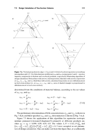
Figure 7.4. Normal projections to edges 1-2 (a,c) and 3-4 (b,d) of section trajectories at nonsharp
intermediatesplit1,2:3,4ofidealmixtureatdifferentx D4 andx B1 (components1and4−non-key
impurity components in bottom and overhead products, respectively) illustrating algorithm of
design calculation. Dotted lines with arrows, trial trajectories; thin lines with arrows, trajectories
at x ◦ D,4 , x ◦ f −1 , x ◦ B,1 and x ; thick lines with arrows, calculated trajectories at zero disbalancement
◦
f
in feed cross-section (i.e., at x D,4 , x f −1 , x B,1 and x f ; area of shaded triangle is proportional to
disbalancement in feed cross-section).
determined from the conditions of material balance, according to the set values
of x F,i , η D , and η B :
F
x D,1 = x F,1 x B,2 = (1 − η B ) − x B,1
D
F B F D
x D,2 = x F,2 − (1 − η B ) x B,3 = x F,3 − (1 − η D ) (7.10)
D D B B
F
x D,3 = (1 − η D ) − x D,4 x B,4 = x F,4
B
The preliminary determination of little concentrations x ◦ and x ◦ is shown in
D,4 B,1
Fig. 7.4a,b, and their specified x D,4 and x B,1 determination is shown in Fig. 7.4c,d.
Figure 7.5 shows the application of this algorithm for equimolar zeotropic
mixture pentane(1)-hexane(2)-heptane(3)-octane(4) at different products pu-
rities η D = η B = 0,999; 0,99; 0,95; 0,9. The values L/V = 1.3(L/V) sh and
min
sh
sh
)
[(x f −1 ) sh − (x ∞ ) ]/[(x min sh − (x ∞ ) ] = 0, 3 were accepted as set parame-
lin f −1 lin f −1 lin f −1 lin
ters of design calculation. One can make out from this figure that, at a sufficiently