Page 106 - Distributed model predictive control for plant-wide systems

80 Distributed Model Predictive Control for Plant-Wide Systems

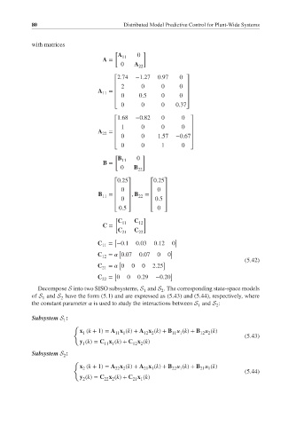
with matrices
[ ]
A 11 0
A =
0 A
22
⎡2.74 −1.27 0.97 0 ⎤
⎢ ⎥
2 0 0 0
A 11 = ⎢ ⎥
⎢ 0 0.5 0 0 ⎥
⎢ ⎥
⎣ 0 0 0 0.37⎦
⎡1.68 −0.82 0 0 ⎤
⎢ 1 0 0 0 ⎥
A = ⎢ ⎥
22
⎢ 0 0 1.57 −0.67⎥
⎢ ⎥
⎣ 0 0 1 0 ⎦
[ ]
B 11 0
B =
0 B 22

⎡0.25⎤ ⎡0.25⎤
0 0
⎢ ⎥ ⎢ ⎥
B 11 = ⎢ ⎥ , B 22 = ⎢ ⎥
⎢ 0 ⎥ ⎢ 0.5 ⎥
⎢ ⎥ ⎢ ⎥
⎣ 0.5 ⎦ ⎣ 0 ⎦
[ ]
C 11 C 12
C =
C C
21 22
[ ]
C 11 = −0.1 0.03 0.12 0
[ ]
C 12 = 0.07 0.07 0 0
(5.42)
[ ]
C = 0 0 0 2.25
21
[ ]
C = 0 0 0.29 −0.20
22
Decompose S into two SISO subsystems, S and S . The corresponding state-space models
1
2
of S and S have the form (5.1) and are expressed as (5.43) and (5.44), respectively, where
2
1
the constant parameter is used to study the interactions between S and S :
1
2
Subsystem S :
1
{
x (k + 1) = A x (k)+ A x (k)+ B u (k)+ B u (k)
11 1
12 2
12 2
11 1
1
(5.43)
y (k)= C x (k)+ C x (k)
1
11 1
12 2
Subsystem S :
2
{
x (k + 1) = A x (k)+ A x (k)+ B u (k)+ B u (k)
2 22 2 21 1 22 1 21 1
(5.44)
y (k)= C x (k)+ C x (k)
2 22 2 21 1