Page 109 - Distributed model predictive control for plant-wide systems

Local Cost Optimization-based Distributed Model Predictive Control 83

LCO−DMPC

4
3.5
3
2.5
2
1.5
1
0.5
3
2
1 25 30
0 20
−1 15
log 10 γ 10
−2
−3 5 P
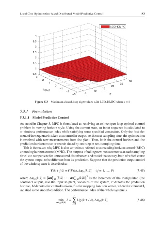
Figure 5.3 Maximum closed-loop eigenvalues with LCO-DMPC when = 1

5.3.1 Formulation
5.3.1.1 Model Predictive Control

As stated in Chapter 3, MPC is formulated as resolving an online open loop optimal control
problem in moving horizon style. Using the current state, an input sequence is calculated to
minimize a performance index while satisfying some specified constraints. Only the first ele-
ment of the sequence is taken as a controller output. At the next sampling time, the optimization
is resolved with new measurements from the plant. Thus, both the control horizon and the
prediction horizon move or recede ahead by one step at next sampling time.
This is the reason why MPC is also sometimes referred to as receding horizon control (RHC)
or moving horizon control (MHC). The purpose of taking new measurements at each sampling
time is to compensate for unmeasured disturbances and model inaccuracy, both of which cause
the system output to be different from its prediction. Suppose that the prediction output model
of the whole system is described as

Y(k + j|k)= f(Y(k), Δu (k|k)) ( j = 1, … , P) (5.45)
M
[ T T ] T
where Δu (k|k)= Δu (k|k) ··· Δu (k|k) is the increment of the manipulated (the
M 1,M m,M
controller output, also the input to plant) variables of the system, P denotes the prediction
horizon, M denotes the control horizon, f is the mapping function vector, where the element f i
satisfied some smooth condition. The performance index of the whole system is
P
∑
min J = L[y(k + l|k), Δu (k|k)] (5.46)
M
Δu M (k|k)
l=1