Page 113 - Distributed model predictive control for plant-wide systems

Local Cost Optimization-based Distributed Model Predictive Control 87

where a (k)(k = 1, … , P; j = 1, … , m) is the sampled output value of the ith subsystem for the
ij
jth subsystem unit step input at the sampling time instant k. The local performance index for
the ith subsystem can be expressed as
2
min J (k)= ‖ (k)− ̃ y i,PM (k)‖ 2 + ‖Δu i,M (k)‖ (i = 1, … , m) (5.53)
i,P
i
Δu i,M (k) Q i R i
where
[ T T ] T
(k)= (k + 1) ··· (k + P)
i
i
i
are the expected output values of the ith subsystem.
̃ y T (k)=[̃ y T (k + 1|k) L ̃ y T (k + P|k)] T
i,PM i,M i,M
T
T
̃ y T (k)=[̃ y (k + 1|k) L ̃ y (k + P|k)] T
i,P0 i,0 i,0
and
Δu T (k)=[Δu (k + 1|k) L Δu (k + M − 1|k)] T
i,PM i,M i,M
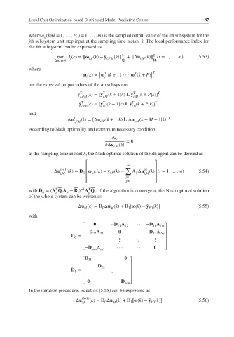
According to Nash optimality and extremum necessary condition
J
i = 0
Δu (k)
i,M
at the sampling time instant k, the Nash optimal solution of the ith agent can be derived as
⎡ ⎤
m
(l+1) ⎢ ∑ (l) ⎥
Δu (k)= D i,P (k) − y (k)− A Δu (k) (i = 1, … , m) (5.54)
ij
i,P
i,M ii ⎢ j,M ⎥
⎢ j=1 ⎥
⎣ j≠i ⎦
T
−1
T
with D =(A Q A + R ) A Q . If the algorithm is convergent, the Nash optimal solution
ii
i
ii
i
i
ii
ii
of the whole system can be written as
Δu (k)= D Δu (k)+ D [ (k)− ̃ y (k)] (5.55)
P0
0
M
1
M
with
−D A ··· −D A
⎡ 11 12 11 1m⎤
−D A 21 ··· −D A 2m
⎢ ⎥
22
22
D = ⎢ ⎥
0
⎢ ⋮ ⋮ ⋱ ⋮ ⎥
⎢ ⎥
⎣−D A ··· · ·· ⎦
mm m1
D
⎡ 11 ⎤
D 22
⎢ ⎥
D = ⎢ ⎥
1
⎢ ⋱ ⎥
⎣ D mm ⎥ ⎦
⎢
In the iteration procedure, Equation (5.55) can be expressed as
(l+1) l
Δu (k)= D Δu (k)+ D [ (k)− ̃ y (k)] (5.56)
P0
0
1
M M