Page 114 - Distributed model predictive control for plant-wide systems

88 Distributed Model Predictive Control for Plant-Wide Systems

At time instant k, (k), and ̃ y (k) are known in advance; hence, D [ (k)− ̃ y (k)] is the con-
P0
1
P0
stant term irrelevant to the iteration. The convergence of expression (5.56) is then equivalent
to that of the following equation:
(l+1) l
Δu (k)= D Δu (k) (5.57)
M 0 M
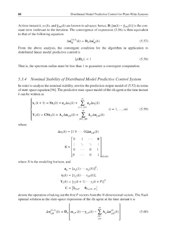
From the above analysis, the convergent condition for the algorithm in application to
distributed linear model predictive control is
| (D )| < 1 (5.58)
0
That is, the spectrum radius must be less than 1 to guarantee a convergent computation.

5.3.4 Nominal Stability of Distributed Model Predictive Control System

In order to analyze the nominal stability, rewrite the prediction output model of (5.52) in terms
of state-space equation [96]. The predictive state-space model of the ith agent at the time instant
k can be written as
m
⎧ ∑
⎪ x (k + 1) = Sx (k)+ a Δu (k)+ a Δu (k)
i
ii
j
ij
i
i
⎪ j=1, j≠i
(i = 1, … , m) (5.59)
⎨ m
∑
⎪
Y (k)= CSx (k)+ A Δu i,M (k)+ A Δu j,M (k)
i
i
ij
ii
⎪
⎩ j=1, j≠i
where
Δu (k)=[10 ··· 0]Δu i,M (k)
i
⎡ 0 1 ··· ⎤
⋮ ⋱ ⋱ ⋮
⎢ ⎥
S = ⎢ ⎥
⎢ 0 ··· 0 1 ⎥
⎢ ⎥
⎣0 ··· 0 1 ⎦
(N×N)
where N is the modeling horizon, and
T
a =[a (1) ··· a (N)] ,
ij
ij
ij
x (k)=[x (k) ··· x (k)],
iN
i
i1
Y (k)=[y (k + 1) ··· y (k + P)] T
i i i
[ ]
C = I
P×P P×(N−P)
denote the operation of taking out the first P vectors from the N-dimensional vectors. The Nash
optimal solution in the state-space expression of the ith agent at the time instant k is
⎡ ⎤
m
∑ (l) ⎥
(l+1)
Δ (k)= D (k) − y (k)− A Δu (k) (5.60)
⎢
i,M ii ⎢ i,P i,P ij j,M ⎥
j=1
⎢ ⎥
⎣ j≠i ⎦