Page 133 - Distributed model predictive control for plant-wide systems

Cooperative Distributed Predictive Control 107

6.2.2.3 Optimization Problem
Problem 6.1 For each independent controller C , i = 1, … , m, the unconstrained C-DMPC
i
problem with the prediction horizon P and control horizon M, M < P, at time k is to minimize
the performance index (6.4) with the system equation constraint (6.5), that is,
P M
∑ i d 2 ∑ 2
min ‖̂ y (k + l|k)− y (k + l|k)‖ + ‖Δu (k + l − 1|k)‖
i
ΔU i (k,M|k) Q R i
l=1 l=1
st. Eq.(7) (6.6)
At time k, based on the exchanged information ̂ x (k|k − 1), U (k + l|k − 1), together with
j
j
x(k), the optimization problem (6.6) is solved in each independent C . The first element of
i
the optimal solution is selected and u (k) = u (k − 1) +Δu (k|k) is applied to S . Then, by
i i i j
Equation (6.5), each local controller estimates the future state at time k + 1 and broadcasts
it in the network together with the optimal control sequence over the control horizon. At time
k + 1, each local controller uses this information to repeat the whole procedure.

6.2.3 Closed-Form Solution
The main result of this subsection is the computation of a closed-form solution to the C-DMPC
problem. For this purpose, the C-DMPC Problem 6.1 is first transformed into a quadratic pro-
gram (QP) problem which has to be locally solved online at each sampling instant.
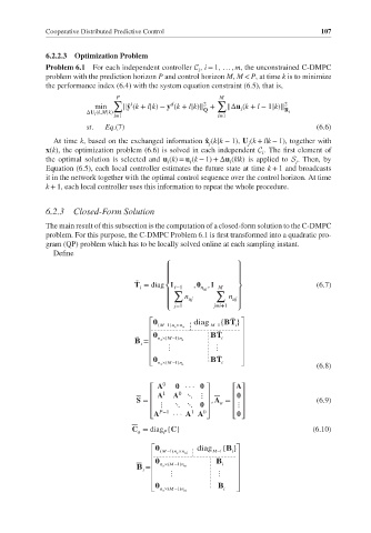
Define

⎧ ⎫
⎪ ⎪
⎪ ⎪
̃
T = diag I , , I (6.7)
i ⎨ i−1 n ui M ⎬
∑ ∑
⎪ ⎪
n uj n uj
⎪ ⎪
⎩ j=1 j=i+1 ⎭
0 (M − 1) x n × n diag M− 1 {BT i }
u
0 (M − BT
B = x n × 1) u n i
i
0 BT
x n × (M − 1) u n i
(6.8)
⎡ A 0 ··· ⎤ ⎡A⎤
⎢ A 1 A 0 ⋱⋮ ⎥ ⎢ ⎥
S = , A = (6.9)
⋮
a
⎢ ⋮ ⋱ ⋱ ⎥ ⎢ ⎥
⎢ P−1 1 0 ⎥ ⎢ ⎥
⎣A ··· A A ⎦ ⎣ ⎦
C = diag {C} (6.10)
a P
B
0 (M − 1) x n × n ui diag M− 1 {}
i
0 (M − n B i
B = x n × 1) ui
i
0 x n × (M − 1) ui B i
n