Page 137 - Distributed model predictive control for plant-wide systems

Cooperative Distributed Predictive Control 111

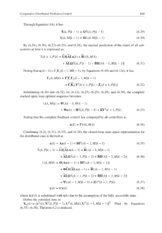
Through Equation (14), it has
X(k, P|k − 1)= (k, P|k − 1) (6.29)
̂
̂
U(k, M|k − 1)= (k, M|k − 1) (6.30)
By (6.29), (6.30), (6.23)–(6.25), and (6.28), the stacked prediction of the states of all sub-
systems at time k is expressed as
(k + 1, P|k)= LS[ALx(k)+ B (k, M|k)
̂
̃
̂
̃
+ AL (k, P|k − 1)+ B (k − 1, M|k − 1)] (6.31)
Noting that u (k − 1) =Γ U (k − 1, M|k − 1), by Equations (6.10) and (6.13e), it has
i
i
i
′
U (k, M|k)= U (k − 1, M|k − 1)
i
i
i i
d
+ K [Y (k + 1, P|k)− Z (k + 1, P|k)] (6.32)
̂
i i i
Substituting (6.16) into (6.32), by (6.12), (6.23)–(6.25), (6.29), and (6.30), the complete
stacked open-loop optimal sequence becomes
(k, M|k)= (k − 1, M|k − 1)
d
+ x(k)+ (k, P|k − 1)+ Y (k + 1, P|k) (6.33)
̂
Noting that the complete feedback control law computed by all controllers is
u(k)= (k, M|k) (6.34)
Combining (6.2), (6.31), (6.33), and (6.34), the closed-loop state-space representation for
the distributed case is derived as

x(k)= Ax(k − 1)+ B (k − 1, M|k − 1) (6.35)
̂
(k, P|k − 1)= LS[ALx(k − 1)+ B (k − 1, M|k − 1)
+ AL (k − 1, P|k − 2)+ B (k − 2, M|k − 2)] (6.36)
̃
̃
̂
(k, M|k)= [Ax(k − 1)+ B (k − 1, M|k − 1)]
+ LS[ALx(k − 1)+ B (k − 1, M|k − 1)
̃
̂
̃
+ AL (k − 1, P|k − 2)+ B (k − 2, M|k − 2)]
d
+ (k − 1, M|k − 1)+ (k + 1, P|k) (6.37)
y(k)= Cx(k) (6.38)
where ̂ x(k|k) is substituted with x(k) due to the assumption of the fully accessible state.
Define the extended state as
T
̂ T
T
T
X (k)=[x (k), X (k, P|k − 1), U (k, M|k), U (k − 1, M|k − 1)] T Then by Equations
N
(6.35)–(6.38), Theorem 6.2 is deduced.