Page 139 - Distributed model predictive control for plant-wide systems

Cooperative Distributed Predictive Control 113

It can be seen that the performance indices in (6.39) and (6.40) are identical. The state
evolution models are also similar. The only difference between these two problems is that,
in C-DMPC, the initial states and future control sequences of other subsystems at time k are
substituted by the estimations calculated at time k − 1. If there is disturbance, model mismatch
or set-point change, the future input sequences of subsystems calculated at time k are not equal
to that calculated at time k − 1, which induces estimation errors of future states between two
optimization strategies. This affects the final performance of the closed-loop system. Although
this difference exists, the optimization problem of C-DMPC is still very close to that of the
centralized MPC.

6.2.5 Example

In this section, the performance of the proposed C-DMPC is investigated and compared with
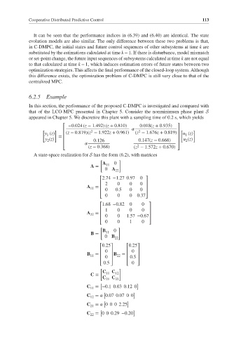
that of the LCO-MPC presented in Chapter 5. Consider the nonminimum phase plant S
appeared in Chapter 5. We discretize this plant with a sampling time of 0.2 s, which yields
⎡ −0.024 (z − 1.492) (z + 0.810) 0.018(z + 0.935) ⎤
[ ] ⎢ 2 2 ⎥ [ ]
y (z) (z − 0.819)(z − 1.922z + 0.961) (z − 1.676z + 0.819) u (z)
1 = ⎢ ⎥ 1
y (z) ⎥ u (z)
2 ⎢ 0.126 0.147(z − 0.668) 2

⎢ 2 ⎥
⎣ (z − 0.368) (z − 1.572z + 0.670) ⎦
A state-space realization for S has the form (6.2), with matrices
[ ]
A 11 0
A =
0 A
22
⎡2.74 −1.27 0.97 0 ⎤
⎢ 2 0 0 0 ⎥
A 11 =
⎢
0 0.5 0 0 ⎥
⎢ ⎥
⎣ 0 0 0 0.37⎦
⎡1.68 −0.82 0 0 ⎤
⎢ 1 0 0 0 ⎥
A =
22 ⎢ 0 0 1.57 −0.67 ⎥
⎢ ⎥
⎣ 0 0 1 0 ⎦
[ ]
B 11 0
B =
0 B
22
⎡0.25⎤ ⎡0.25⎤
⎢ 0 ⎥ ⎢ 0 ⎥
B 11 = B 22 =
0 ⎥ ⎢ 0.5 ⎥
⎢
⎢ ⎥ ⎢ ⎥
⎣ 0.5 ⎦ ⎣ 0 ⎦
[ ]
C 11 C 12
C =
C 21 C 22
[ ]
C = −0.10.03 0.12 0
11
[ ]
C 12 = 0.07 0.0700
[ ]
C 21 = 0002.25
[ ]
C 22 = 000.29 −0.20